A Simple Approach to Evolutionary Multi-Objective Optimization Christine L. Mumford-Valenzuela School of Computer Science Cardiff University United Kingdom
[email protected] Summary. This chapter describes a Pareto-based approach to evolutionary multiobjective optimization, that avoids most of the time consuming global calculations typical of other multi-objective evolutionary techniques. The new approach uses a simple uniform selection strategy within a steady-state evolutionary algorithm (EA) and employs a straightforward elitist mechanism for replacing population members with their offspring. Global calculations for fitness and Pareto dominance are not needed. Other state-of-the-art Pareto-based EAs depend heavily on various fitness functions and niche evaluations, mostly based on Pareto dominance, and the calculations involved tend to be rather time consuming (at least O(N 2 ) for a population size, N ). The new approach has performed well on some benchmark combinatorial problems and continuous functions, outperforming the latest state-of-the-art EAs in several cases. In this chapter the new approach will be explained in detail.
Key words: Evolutionary algorithm, Multi-objective optimization, Pareto set, Knapsack problem .
1 Introduction This chapter concentrates on a simple approach to evolutionary multi-objective optimization that avoids most of the time consuming global calculations typical of many other Pareto-based evolutionary approaches. The basic algorithm described here is called SEAMO (a Simple Evolutionary Algorithm for Multiobjective Optimization), and although this new technique has not as yet been very widely tested, it has proven successful on some benchmark combinatorial problems and continuous functions, outperforming other state-of-the-art evolutionary algorithms (EAs) in several instances [19]. In addition to fast execution, the simplicity of the new algorithm makes it relatively quick and easy to implement, reducing the development time needed for prototyping and testing new multi-objective applications. If required, more sophisticated
Pareto-based evolutionary techniques can be incorporated following an initial proof-of-concept. The main purpose of the chapter is to introduce and explain the key concepts involved in the new approach using some simple applications as examples. In addition, in order to justify the approach, a summary of some preliminary comparative studies will be included. I will begin in Section 2 with a brief overview of Pareto-based multiobjective optimization, moving on to multi-objective evolutionary techniques in Section 3. Section 3 also includes a short preview of SEAMO, concentrating on its main features and explaining how it differs from other evolutionary approaches. Following this, Section 4 describes the multiple knapsack problem and introduces a sample test problem with two knapsacks. Section 5 describes the SEAMO algorithm in detail and this is followed, in Section 6 by an illustration of SEAMO’s operation through the test problem introduced in Section 4. Section 7 summarizes SEAMO’s performance on some large multiple knapsack problems. Having studied a combinatorial application, I will turn my attention, in Section 8, to explaining how the techniques can be adapted to handle some continuous multi-objective functions. Some results for the continuous functions are summarized in Section 9. Full details of the representations and genetic operators are given for the combinatorial and continuous problems.
2 Pareto-Based Multi-Objective Optimization Many real-world applications require the simultaneous optimization of several (often competing) objectives. For example, in the vehicle routing problem (VRP) the determination of optimum delivery routes to a set of customers can involve a number of different objectives (Figure 1), for example the total distance travelled (or time taken), the number of vehicles used, and the number of satisfied customers (i.e. deliveries that have taken place to customers within previously agreed time windows). There are three principle methods of dealing with multiple objectives: 1. Combine all the objectives into a single scalar value, typically as a weighted sum, and optimize the scalar value. 2. Solve for the objectives in a hierarchical fashion, optimizing for a first objective then, if there is more than one solution, optimize these solutions for a second objective, and repeat for a third etc. if appropriate. 3. Obtain a set of alternative, non-dominated solutions, each of which must be considered equivalent in the absence of further information regarding the relative importance of each of the objectives. The first and the second methods both depend on making a priori assessments to weigh up the relative importance of the various objectives. The third method, on the other hand, involves no such (arbitrary) judgments, and produces a set of viable alternatives from which a decision maker can make
Fig. 1. Vehicle routing can be a problem
an informed selection at a later stage. Ideally each alternative solution produced by method 3 will be optimal in the sense that it will not be possible to improve the value of any one of the objectives, in a given solution vector, without simultaneously degrading the quality of one or more of the other objectives. Such a solution set is called the Pareto-optimal set, and the objective values in the set are located at the Pareto front. SEAMO is an evolutionary algorithm that has been designed to produce approximate Pareto sets. Thus method 3 is the way we will deal with multiple objectives in the remainder of this chapter.
3 An Overview of Evolutionary Techniques for Multi-Objective Optimization Evolutionary algorithms (EAs) are ideally suited for multi-objective optimization problems because they produce many solutions in parallel. However, traditional approaches to EAs require scalar fitness information and converge on a single compromise solution, rather than on a set of viable alternatives. An
effective Pareto-based multi-objective EA will converge on a solution set with the following properties: • • •
solutions that are ‘good’, i.e. close to the Pareto front solutions that are ‘evenly spread’ along the Pareto front solutions that are ‘widely spread’ - i.e. a good range
To seek solution sets with the above properties, most researchers rely on selection that uses some form of Pareto-based fitness assignment. This idea, which was first proposed by Goldberg [8], is based on dominance ranking and assigns equal probability of reproduction to all non-dominated individuals. Solutions can be further improved using techniques such as fitness sharing [8], niches [6, 10] and auxiliary populations [2, 21]. Unfortunately most of these approaches carry a high computational cost. The present approach relies on very much simpler techniques. It disposes of all selection mechanisms based on fitness values and instead uses a straightforward uniform selection procedure (i.e. each population member has an equal chance of being selected). Thus no dominance ranking is required. In the new approach improvements to the population and progress of the genetic search depend entirely upon a replacement strategy that follows a few simple rules: 1. parents are (normally) replaced only by their own offspring, 2. offspring only replace parents if the offspring are superior – thus the scheme is elitist, 3. duplicates in the population are deleted. SEAMO depends on rules 1 and 3 to maintain diversity and prevent premature convergence and on rule 2 to progress the genetic search and also ensure that the best solutions are not lost. Replacing parents only with their own offspring (rule 1) means that the new individuals tend to be genetically very similar to the population members they are replacing. Alternative replacement schemes, on the other hand (replacing one of the weaker members of the population for example) can lead to a much more rapid propagation of duplicated genetic material, and thus to premature convergence. SEAMO further promotes genetic diversity by deleting duplicates (rule 3) as soon as they arise in the population. Ideally an EA should discard genotypic duplicates. (A genotypic duplicate is an individual with exactly the same genetic makeup as another individual.) Unfortunately the pairwise comparisons between chromosomes needed to detect genotypic duplicates tends to be rather time consuming unless the chromosomes are very short. Current implementations of SEAMO delete phenotypic duplicates, i.e. individuals with the same solution vectors as other individuals. As the solution vectors are usually rather shorter than the chromosomes, this tends to be a very much faster process. Deleting phenotypic duplicates will certainly eliminate genotypic copies. Unfortunately it can also lead to the deletion of genetically diverse individuals if, by chance, they produce identical solution vectors. In practice this does not seem to arise very often though.
Rule 2 controls the overall progress of the genetic search, and ensures that the population as a whole improves over time (hence ensuring that solutions are ‘good’). A ‘superior’ offspring in rule 2 is defined (most of the time) as an offspring that dominates one or other of its parents (i.e. one of the objectives in its solution vectors is better than its parent, and all the other objectives are at least as good). An exception is made when an offspring arises with a new global best value for just one of the objectives in its solution vector. When this occurs, the dominance condition is relaxed, and the new individual is assimilated into the population (hence ensuring that solutions are ‘widely spread’). The new individual usually replacing one of its parents (this will be explained in Section 5). Rule 2 ensures that the EA itself is elitist, thus, unlike [2] and [21] no archive population is needed. We shall see later in this chapter that SEAMOs subtle techniques appear to work well in producing solutions that both ‘good’ and ‘widely spread’, and thus meet two of the three criteria for effective Pareto-based EAs specified at the start of the current section. However, current implementations of SEAMO lack a specific mechanism to ensure that the solutions are ‘evenly spread’, and this can cause difficulties when applying SEAMO to certain functions. In common with other EAs, successful multi-objective implementations require well-designed representation systems for individual problems and also genetic operators that are appropriate for the task. Recombination (crossover) operators can be particularly problematic. At worst an EA may waste vast quantities of time generating invalid or illegal offspring, and even in a superficially successful system, a crossover may produce an offspring that bears very little phenotypical resemblances to either of its parents. As the similarity between parents and their offspring remains one of the main tenets of evolution, a poorly designed or inappropriate recombination operator can turn an otherwise perfect EA into an implementation that is no more effective than a random search. Unfortunately there does not appear to be a known recipe for producing effective representation schemes, either for single or multi-objective EAs. Experience and intuition can help, but provide no guarantees! Thus the success of SEAMO, or any other EA (multi-objective or otherwise) on a particular application, depends very much on the representation scheme chosen for the application. Additionally it is necessary to tune various parameters of the EA such as population size, crossover and mutation rates, to produce a good performance. Assessing the performance of EAs can be very difficult in practice. Even when the same data sets are used to compare EAs with each other or with alternative approaches, it can be dangerous to draw firm conclusions as to which algorithm is the best. In addition to making sound (or unsound) choices for representations and genetic operators, there are many other issues to consider, and choices to be made. How long do you let the the EAs run? What population sizes and crossover rates do you set? Some EAs converge quickly, while others take longer but produce better results in the end. The algorithms are differently sensitive to parameter settings such as population sizes and
crossover rates, so it is not easy to ensure fairness, especially when comparing an unfamiliar EA that somebody else has written with one of your own (that you would obviously like to win). Notwithstanding the difficulties associated with representations, varying convergence rates and parameter settings, comparisons between EAs (or other metaheuristic approaches such as simulated annealing) are frequently based on each algorithm performing an equal number of fitness or objective function evaluations. This is a very crude method, however, as it ignores important run time issues such as time complexity. Comparisons between EAs that carry out multi-objective optimizations are even more problematic. Here we have the added difficulty of assessing the quality of a each algorithm by examining a set of vectors, instead of examining the single scalar value obtained from a ‘standard EA’. Although a range of performance measures have been derived by various researchers, there is no general agreement upon their usefulness. For vectors consisting of just two objectives it is possible to represent the results quite effectively using 2D plots, and comparisons can be made quite easily if plots for a small number of different algorithms are placed on the same diagram, provided that not too many of the points overlap.
4 The 0-1 Multiple Knapsack Problem
Fig. 2. The same objects may have different weights in each knapsack
Fig. 3. The same objects may have different profits in each knapsack
The 0-1 multiple knapsack problem (0-1 MKP) is a maximization problem. It is a generalization of the 0-1 simple knapsack problem, and is a well-known member of the NP-hard class of problems. In the simple knapsack problem, a set of objects O = {o1 , o2 , o3 , ..., on } and a knapsack of capacity C are given. Each object oi has an associated profit pi and weight wi . The objective is to find a subset S ⊆ O such that the weight sum over the objects in S does not exceed the knapsack capacity and yields a maximum profit. The 0-1 MKP involves m knapsacks of capacities c1 , c2 , c3 , ..., cm . Every selected object must be placed in all m knapsacks, although neither the weight of an object oi nor its profit is fixed, and will probably have different values in each knapsack (see Figures 2 and 3). A small problem with 10 objects and two knapsacks is defined in Table 1. A possible solution to the ten object, two knapsack problem from Table 1 is {2, 3, 4, 5, 6, 7, 9}, which involves packing objects number 2, 3, 4, 5, 6, 7 and 9 into the two knapsacks. To evaluate the solution vector for this problem requires that we first ensure that neither knapsack capacity has been exceeded. The total weight of the given objects when packed into knapsack 1 is 8+2+7+ 3+6+1+9 = 36 units, and in knapsack 2 they weigh 4+2+4+9+5+4+3 = 31 units. In neither case is the knapsack capacity (38 and 35) exceeded. We then work out the total profit for each knapsack by adding together the profits for each of the items packed. The total profit in knapsack 1 is 7 + 4 + 5 + 6 + 2 + 7 + 7 = 38, and in knapsack 2 is 9 + 1 + 5 + 3 + 8 + 2 + 1 = 29. The solution {2, 3, 4, 5, 6, 7, 9} yields a solution vector of {38, 29}, the profits in knapsacks 1 and 2 respectively. The full Pareto set, for this small problem, is presented in Table 2. The solutions were discovered using a simple exhaustive search technique which took only a few seconds to run.
Table 1. A sample problem with ten objects and two knapsacks Knapsack 1 Knapsack 2 Object number Capacity = 38 Capacity = 35 Weight Profit Weight Profit 1 2 3 4 5 6 7 8 9 10
9 8 2 7 3 6 1 3 9 3
2 7 4 5 6 2 7 3 7 1
3 4 2 4 9 5 4 8 3 7
3 9 1 5 3 8 2 6 1 3
Table 2. The Pareto set for the sample problem with ten objects and two knapsacks Knapsack 1 Profit knapsack 2 Profit Objects in Knapsacks 39 38 36 35 34 32 29 27
27 29 30 32 33 34 35 36
{2, 3, 4, 5, 7, 8, 9} {2, 3, 4, 5, 6, 7, 9} {2, 3, 5, 6, 7, 8, 9} {2, 3, 4, 6, 7, 8, 9} {2, 3, 4, 5, 6, 8, 9} {2, 4, 6, 7, 8, 9, 10} {1, 2, 3, 4, 5, 6, 8} {1, 2, 4, 6, 7, 8, 10}
5 An Introduction to SEAMO The Simple Evolutionary Algorithm for Multi-objective Optimization (SEAMO), is outlined in Figure 4. The goal of any Pareto-based multi-objective EA is to breed a widely and evenly spread population of solution vectors, as close to the Pareto front as possible. The dual aims pursued by SEAMO during its search process are: (1) to move the current solutions in the population ever closer to the Pareto front, and (2) to widen the spread of the solution set. Improvements in both (1) and (2) are achieved by the replacement strategy used in SEAMO, and not by the selection process. It was noted previously that SEAMO currently has no specific mechanism for ensuring that the solutions are evenly spread. The selection procedure for SEAMO is very simple and does not rely on fitness calculations or dominance relationships. The crossover rate is 100 %, which means that parents are always selected in pairs. The algorithm sequentially selects every individual in the population to serve as the first parent once, pairing it with a second parent that is selected at random (uniformly).
Procedure SEAMO Begin Generate N random individuals {N is the population size} Evaluate the objective vector for each population member and store it Record the global best-so-far for each objective function in the vector Repeat For each member of the population This individual becomes the first parent Select a second parent at random Apply crossover to produce offspring Apply a single mutation to the offspring Evaluate the objective vector produced by the offspring If any element of the offspring’s objective vector improves on a global best-so-far Then the offspring replaces one of the parents (or occasionally another individual) and best-so-far is updated Else If offspring dominates one of the parents Then it replaces it (unless it is a duplicate, then it is deleted) Endfor Until stopping condition satisfied Print all non-dominated solutions in the final population End Fig. 4. Algorithm 1 A Simple Evolutionary Algorithm for Multi-objective Optimization (SEAMO)
A single crossover is then applied that produces one offspring, and this is followed by a single mutation. Objective values and dominance relationships are not considered at this stage. They are applied later, at the replacement stage, and it is here, rather than during selection, that the pressure for improvement is applied. As explained previously, the replacement of a parent by its offspring is considered whenever an offspring is deemed to be superior to that parent. This idea, called pre-selection when it was first suggested in [1], was originally used for EAs with scalar objective functions. The technique easily extends to Pareto-based multi-objective optimization, however. In the SEAMO algorithm, the superiority test is applied first of all to the first parent, and then to the second parent if that fails. Usually superiority is measured as a dominance relationship, i.e. if an offspring dominates its parent, it may replace it in the population. The replacement of population members by dominating offspring ensures that the solution vectors move closer to the Pareto front as the search progresses. To additionally ensure a wider spread of solutions, the dominance condition is relaxed whenever a new global best value is discovered
for any of the individual components of the solution vector. In the case of the multiple knapsack problem for example, a global best value will correspond to a maximum profit in one of the m knapsacks. Care has to be taken, however, to ensure that global best values for other components (e.g. maximum profits in other knapsacks) are not lost from the population when a dominance condition is relaxed. Ensuring elitism (i.e. that the best solutions are not lost) at this level is straightforward if multi-objective optimization is restricted to two components in the solution vector. Whenever an offspring produces an improved global best for either of the components, if the global best for the second component happens to occur in one of the parents, the offspring will simply replace the other parent. With three or more components, however, it is possible for global best values to occur in both parents. When this happens SEAMO replaces another population member, chosen at random, provided that the newly selected individual does not itself harbor a global best. If it does, the random selection process is repeated until a suitable individual is found. As a final precaution, a solution vector for a dominating offspring is compared with all the solution vectors in the current population before a final decision is made on replacement. If the solution vector produced by the offspring is duplicated elsewhere in the population, the offspring dies and does not replace its parent. As previously mentioned, the deletion of duplicates helps maintain diversity in the population and thus avoid the premature convergence of the population to sets of identical, or very similar, individuals. The final action of SEAMO is to save all the non-dominated solutions from the final population to a file.
6 Illustrating SEAMO Using a Small Multiple Knapsack Problem Several approaches have been suggested for representing solutions to single objective knapsack problems for EAs. Michalewicz [13] identifies three classes: algorithms based on penalty functions , algorithms based on repair methods , and algorithms based on decoders (i.e. interpreters to convert lists of symbols in the chromosomes into solutions to the required problem). The main challenge with the knapsack problem is to ensure that the EA does not waste vast amounts of its time in generating illegal solutions with over-full knapsacks. In the present study, SEAMO uses a representation system based on a decoder for the 0-1 MKP. (Experiments with other representations for the 0-1 MKP are documented in a later study by the present author, see [15]). For the decoder scheme MKP solutions are represented as simple permutations of the objects to be packed. The decoder packs the individual objects, one at a time, starting at the beginning of the permutation list, and working through. For each object that is packed, the decoder checks to make sure that none of the weight limits is exceeded for any knapsack. Packing is discontinued as
Fig. 5. Packing is discontinued and the final item removed as soon as the weight limit is exceeded for a knapsack
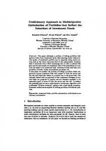
soon as a weight limit is exceeded for a knapsack (Figure 5) and when this is detected the final object that was packed is removed from all the knapsacks. Thus, each knapsack contains exactly the same objects as required, and each solution that is generated is a feasible solution. Using the ten object problem with two knapsacks given previously as an example, given a permutation of {2,5,1,7,9,8,10,3,4,6}, the decoder would first pack item 2, which weighs 8 units in knapsack 1 and 4 units in knapsack 2. Item 5 would be packed next, weighing 3 units in knapsack 1 and 9 units in knapsack 2, giving total weights of 11 and 13 for the two knapsacks. The decoder would carry on packing items from the permutation list until it had packed item 10, giving total weights of 36 and 39 for knapsacks 1 and 2 respectively. A weight of 39 units in knapsack 2 exceeds the capacity of the knapsack, and so the last item to be packed, which is item 10, is removed from both knapsacks giving final weights of 33 units for knapsack 1 and 31 units for knapsack 2. The profit vector for packing the items 2, 5, 1, 7, 9, and 8 is {32, 24}. Cycle crossover (CX) [16] is used as the recombination operator with the above permutation representation, and the mutation operator swaps two arbitrarily selected objects within a single permutation list. Cycle crossover was selected as the recombination operator because it transmits absolute positions of objects in the permutation lists from the parents to the offspring. Neither edge based nor order based operators would seem to be appropriate here, for a set membership problem such as this. Some comparative runs shown in Figure 6 support the choice of CX as the recombination operator. This figure compares the performance of four different permutation-based operators on a 750 object, 2 knapsack problem (see Section 7). The traces on Figure 6 are
4
3
Plots for 750 objects in 2 knapsacks
x 10
PMX CX OX UOBX
Profit in second knapsack
2.9
2.8
2.7
2.6
2.5
2.4 2.4
2.5
2.6
2.7 Profit in first knapsack
2.8
2.9
3 4
x 10
Fig. 6. Non-dominated solutions for different crossovers
partially matched crossover (PMX) [7], cycle crossover (CX) [16], a version [14] of order crossover (OX) [4] that preserves absolute positions better than the original, and uniform order based crossover (UOBX) [5]. Populations of 250 were used for the test runs, and the EA run for 15,000 generations. Clearly the plot of SEAMO using CX gives a much more diverse set of solutions than any of the other plots. However, the UOBX solutions, although considerably less diverse than the CX solutions, are slightly better in quality. 6.1 Cycle Crossover The cycle crossover operator ensures that each position in the resulting offspring is occupied by a value occupying the same position in one or other of the parents. As an example, suppose we have strings A and B below as our two parents:
A =8 B =2
7 5
6 1
4 7
1 3
2 8
5 4
3 6
9 10 10 9
We now start from the left and randomly select an item from string A. Suppose we choose item 6 from position 3, this is then copied to position 3 of the offspring we shall call A′ : A′ = –
–
6
–
–
–
–
–
–
–
In order to ensure that each value in the offspring occupies the same position as it does in either one or other parent, we now look in position 3 of string B and copy item 1 from string A to the offspring: A′ = –
–
6
–
1
–
–
–
–
–
Next we look in position 5 of string B and copy item 3 from string A: A′ = –
–
6
–
1
– –
3 –
–
Looking at position 8 in string B we find item 6. This completes the cycle. We now fill the remaining positions in A′ from string B thus: A′ = 2 B′ = 8
5 7
6 1
7 4
1 3
8 4 2 5
3 10 9 6 9 10
The offspring B ′ is obtained by performing the complementary operations.
7 A Summary of Results for Multiple Knapsack Problems The multiple knapsack problems of Zitzler and Thiele [21] were used as the first set of test problems for SEAMO. These were a convenient choice because of the extensive comparative studies that had already been carried out on these problems, covering a wider range of state-of-the-art EAs (see [21] and [22] for details). Furthermore, Zitzler and Thiele have made their test problems and most of their key results available at: http://www.tik.ee.ethz.ch/zitzler/testdata.html.
7.1 Comparisons With Other Evolutionary Algorithms In [19] SEAMO was compared with SPEA [21] (the strength Pareto evolutionary algorithm) , and was found to do better. However, when SEAMO was compared with the more recent EAs covered in [22], PESA (the Pareto envelope-based seletion algorithm) [2], NGSA2 (a fast elitist non-dominated sorting genetic algorithm) [3], and SPEA2 an improved version of SPEA (the strength Pareto evolutionary algorithm) SPEA (the strength Pareto evolutionary algorithm) [21], it found these results more difficult to beat. Interestingly, though, SEAMO improved its performance, relative to the other EAs as more knapsacks (i.e. objective functions) were added. For a large problem with 750 objects, for example, SEAMO was easily beaten by some other EAs using the same populations sizes and running the algorithms for the same number of generations, when only 2 knapsacks were used. SPEA2 [22] produced particularly impressive results on this problem. When tested on a 750 object problem with 3 knapsacks, SEAMO performed much better, relative to the other EAs, although not quite able to match the other EAs on an evaluation for evaluation basis. For the 750 object problems with either 2 or 3 knapsacks, SEAMO is able to beat its competitors only if it is allowed to perform more evaluations. Given the simplicity of the SEAMO algorithm, however, it may be acceptable that it performs more evaluations, depending how much faster it runs than its competitors. On the other hand, for the problem with 750 objects and 4 knapsacks, SEAMO was easily able to outperform all its main competitors performing the same number of evaluations. 7.2 The Effect of Increasing the Population Size In order to shed further light on the effect of increasing the number of evaluations performed by SEAMO, a number of single runs were carried out on a 750 object, 2 knapsack problem using various sizes of population. Figure 7 illustrates the results of some of these experiments. Population sizes of 100, 200, 500, 1,000, 2,000 and 5,000 were tried and the EA halted after 40 generations have elapsed in which no improvements have been made to the population. Clearly, increasing the population size produces better results, consisting of a larger quantity of non-dominated solutions which are closer to the Pareto front. However the improvements are fairly small between population sizes of 500 and 5,000. Surprisingly, perhaps, the SEAMO run with a population of 100 appears to produce a wider spread of results, than the runs with the larger populations. Some key features of all the runs are presented in Table 3. Columns two and three of Table 3 give the total number of evaluations and the run time, respectively. Column four gives the number of non-dominated solutions present in the population at the end of each run. The size of this nondominated set clearly gets larger as the population is increased. Columns five and six give the smallest and largest profits found in the final non-dominated set for each knapsack. As previously suggested, the range of values would
4
3
Plots for 750 objects in 2 knapsacks
x 10
Population = 100 Population = 500 Population = 5000 2.9
Profit in second knapsack
2.8
2.7
2.6
2.5
2.4
2.3 2.4
2.5
2.6
2.7 Profit in first knapsack
2.8
2.9
3 4
x 10
Fig. 7. Non-dominated solutions from single runs of SEAMO showing the effect of increasing the population size
Table 3. The effect on SEAMO of increasing population size Population Run time Number of Largest Largest Total size Evaluations (secs) non-dom. solns. profit 1 profit 2 100 200 500 1,000 2,000 5,000
950,900 2,605,000 4,154,000 13,956,000 32,118,000 151,250,000
154 442 777 2,705 6,356 30,603
56 79 103 176 237 260
29,589 29,543 29,134 29,255 29,334 29,141
29,585 29,555 29,192 29,318 29,069 29,504
appear to decrease slightly as the population size is increased. A possible explanation for this could be that smaller populations are more focussed towards widening the spread of solutions than larger populations, because the dominance condition for parental replacement is likely to be relaxed, a higher proportion of the time, in order to incorporate new global best-so-far objective values.
4
3
Plots for 750 objects in 2 knapsacks
x 10
Dominance and global best Dominance only Global best only
2.9
Profit in second knapsack
2.8
2.7
2.6
2.5
2.4
2.3
2.2
2.1 2.1
2.2
2.3
2.4
2.5 2.6 Profit in first knapsack
2.7
2.8
2.9
3 4
x 10
Fig. 8. Results showing the effect of using one or other or both replacement criteria
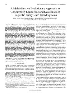
7.3 Investigation of SEAMO’s Parental Replacement Strategy Progress in SEAMO is due entirely to its replacement strategy. Recall from Section 5 that an offspring will replace one or other of its parents if it is deemed to be superior to that parent. Most replacements occur when an offspring dominates one of its parents. However, in situations where a new global best value is discovered for one of the positions in the solution vector, the dominance condition is relaxed, to encourage a wider spread of approximate Pareto solutions within the population. In this section I investigate the contribution of each component in the replacement strategy with some experimental runs. In the first run, both replacement components are present. In the second run, parents are replaced only by dominating offspring and not when new global best values are discovered (unless the offspring solution with the new global best also dominates a parental solution). The third run shows the effect of replacing parents only when new global best values are discovered. The 750 object, 2 knapsack problem is used for the experiments, and the population size set to 500. All three tests are run for 13504 generations. The results are plotted in Figure 8. Clearly, using both the replacement strategies together produces the best results by far. Replacing parents only by dominating offspring appears to produce high quality solutions, but within a very
limited range. Replacing parents only with offspring that improve a global best value at any position in the solution vector, produces very poor solutions, and very few of them.
8 Implementing SEAMO to Solve Continuous Test Problems
Fig. 9. Continuous multi-objective functions
Having completed some preliminary work testing SEAMO on multiple knapsack problems, I then tried SEAMO on some continuous test functions, published in [22]. The permutation representation and decoder used for the knapsack problems is not suitable for continuous functions, so a different scheme had to be devised. The continuous functions and their parameters are summarized in Table 4. Each of the test problems in Table 4 is a minimization problem consisting of two objectives and 100 variables. For SPH-2 and KUR large domains ([−103 , 103 ]) were selected in [22] in order to test the algorithms’ ability to locate the Pareto-optimal set in a large objective space. The function SPH-m is a multi-objective generalization of the Sphere Model, a symmetric unimodal function where the isosurfaces are given by hyperspheres. Only the two objective instance (SPH-2) is covered in the present paper, although Zitzler et al [22] also included the three objective instance in their experiments.
Table 4. Continuous test problems used in this study. The objective functions are given by fj , 1 ≤ j ≤ m, where m denotes the number of objectives and n the number of variables. The type of the objectives is given in the first column (minimization or maximization). n Domain Objective functions Type SPH-m (Schaffer 1985 [?]; Laumans, Rudolph, and Schwefel 2001, [12]) 100 min
∑
[−103 , 103 ]n fj (x) = 1≤i≤n,i̸=j (xi )2 + (xj − 1)2 1 ≤ j ≤ m, m = 2 ZDT6 (Zitzler, Deb and Thiele 2000, [20])
100 min
[0, 1]
f1 (x) = 1 − exp(−4x1 )sin6 (6πx1 ) f2 (x) = g(x)[1 ∑ − (f1 (x)/g(x))2 ] n g(x) = 1 + 9.(( i=2 xi /(n − 1)))0.25
n
QV (Quagliarella and Vicini 1997, [17]) 100
[−5, 5]
n
min
∑n
f1 (x) = (1/n ∑i=1 (x2i − 10 cos(2πxi ) + 10))1/4 n f2 (x) = (1/n i=1 ((xi − 1.5)2 − 10 cos(2π(xi − 1.5)) + 10))1/4 KUR (Kursawe 1991, [11])
100 min
3
3 n
[−10 , 10 ] f1 (x) = f2 (x) =
∑n
i=1
3 (|xi |0.8 + 5. sin √ (xi ) + 3.5828)
∑n−1 i=1
−0.2
(1 − exp
x2 +x2 i i+1
)
ZDT6 is also unimodal and has a non-uniformly distributed objective space, both orthogonal and lateral to the Pareto-optimal front. ZDT6 was proposed in [22] to test the ability of the various algorithms to find a good distribution of points even in this very difficult case. The components of the function QV are two multi-modal functions, where the main difficulty, apart from the multi-modality, is the extreme concave Pareto-optimal front together with a diminishing density of solutions towards the extreme points. Kursawe’s function (KUR) finally has a multi-modal function in one component and pair-wise interactions among the variables in the other component. The Pareto-optimial front is not connected and has an isolated point as well as concave and convex regions. For all of the continuous functions the solutions were coded as real vectors, of length 100, for SEAMO and uniform crossover [18] selected as the recombination operator. Uniform crossover was chosen because the lack of any particular relationship between adjacent variables on the chromosome would seem to reduce any potential advantage that could be obtained by the building blocks created using one or two point crossover (although experiments I carried out later indicate that, in fact, one point crossover produces better results on these continuous functions). For the mutation operator a simple
uniform mutation operator was tried initially, but this was found to be much too disruptive, particularly when large objective spaces were used. For ZDT6 and KUR, for example, individual mutated variables could take any value in the range [−103 , 103 ], and this made convergence of the EA very difficult. To overcome this problem, which is commonplace with real valued representations, a non-uniform mutation based on that described on page 111 of [13] was chosen. The idea of non-uniform mutation is to gradually reduce the magnitude of any change that the operator is allowed to make to the values of the variables as the EA progresses. Non-uniform mutation causes the operator to search the space uniformly initially and very locally at later stages. The nonuniform mutation is defined as follows: if stv = ⟨v1 , . . . , vm ⟩ is a chromosome in the population at time t, and the element vk is selected for this mutation (domain of vk is [lk , uk ]), the result is a vector st+1 = ⟨v1 , . . . , vk′ , . . . , vm ⟩, v with k ∈ {1, . . . , n}, and vk′
{ =
vk + ∆(t, uk − vk ) if a random digit is 0, vk − ∆(t, vk − lk ) if a random digit is 1,
where the function ∆(t, y) returns a value in the range [0, y] such that the probability of ∆(t, y) being close to 0 increases as t increases. The following function has been used in the present study: ∆(t, y) = y.(1 − rf (t) ) where r is a random number from [0 . . . 1], t is the number of generations that have elapsed so far. f (t) = k t is used for these experiments, where k is a constant factor set to 0.999. An important feature of the SEAMO algorithm is the deletion of duplicates, designed to help maintain diversity and prevent premature convergence. For the knapsack problem, and other combinatorial problems, where the objective functions can take on only limited number of discrete values, phenotypic duplicates are easily identified as individuals with identical solution vectors. With continuous functions, however, it is sensible to identify duplicates in a rather more flexible manner, because exact duplicates are likely to be rare. To this end, values for component objective functions xi and x′i are deemed to be equal if and only if xi − ϵ ≤ x′i ≤ xi + ϵ, where ϵ is an error term, which was set at 0.00001 × xi for the purpose of these experiments.
9 Summary of Results for the Continuous Functions Figures 10, 11, 12 and 13 compare the 2D graphical traces of SEAMO with various state-of-the-art EAs on the four continuous problems, respectively SPH-2, ZDT6, QV and KUR. SEAMO’s competitors in the 2D plots are PESA, NGSA2, and SPEA2. Population sizes of 100 were used in each case
and the algorithms run for 10,000 generations. Each trace is a plot of the non-dominated solutions extracted from the results of 30 replicated runs. Note that all the function optimization problems used in this study are minimization problems, unlike the multiple knapsack problem. Thus the algorithms producing the lowest traces on these graphs perform best for the continuous functions. The 2D graphical representations indicate that SEAMO performs very well in comparison with its competitors for three out of four of the continuous functions, i.e. SPH-2, QV and KUR. Table 5 compares the evolutionary algorithms in pairs using values for the C metric defined in [21]. The C metric is measures the coverage of two sets of solution vectors. Let X ′ , X ′′ ⊆ X be two sets of solutions vectors. The function C maps the ordered pair (X ′ , X ′′ ) to the interval [0, 1] C(X ′ , X ′′ ) =
| {a′′ ∈ X ′′ ; ∃ a′ ∈ X ′ : a′ ≽ a′′ } | | X ′′ |
(1)
The value C(X ′ , X ′′ ) = 1 means that all the points in X ′′ are dominated by or equal to points in X ′ , (i.e. all the points in X ′′ are weakly dominated by points in X ′ ). The opposite, C(X ′ , X ′′ ) = 0, represents the situation when none of the points in X ′′ is weakly dominated by X ′ . Note that both C(X ′ , X ′′ ) and C(X ′′ , X ′ ) have to be considered, since C(X ′ , X ′′ ) is not necessarily equal to 1 − C(X ′′ , X ′ ) (i.e. when many solutions in X ′ and X ′′ neither dominate nor are they dominated by solutions in the alternative set). The C metric values used in the table indicate superior coverage of the search space by SEAMO for SPH-2, QV and KUR. Single runs of SEAMO on the continuous functions took between 81 secs for SPH-2, and 412 secs for KUR, using a Pentium III processor and 128 MB of memory. Table 5. C metrics to compare SEAMO with PESA, NSGA2, and SPEA2. The nondominated solutions are collected from 30 results files for each algorithm, as before. A population size of 100 is used and a total of 1,000,000 evaluations is carried out for each run of each algorithm. C(alg1,alg2) C(SEAMO, PESA) C(PESA, SEAMO) C(SEAMO, NSGA2) C(NSGA2, SEAMO) C(SEAMO, SPEA2) C(SPEA2, SEAMO)
SPH-2 99 % 0% 99 % 0% 99 % 0%
ZDT6 0% 93.3 % 0% 93.3 % 0% 93.3 %
QV 94.3 % 0.03 % 63.0 % 0.6 % 58.2 % 0.6 %
KUR 54.9 % 4.9 % 66.3 % 2.0 % 70.4 % 2.1 %
1,000,000 evaluations for SPH−2 2.5 PESA NSGA2 SPEA2 SEAMO 2
f2(x)
1.5
1
0.5
0
0
0.5
1
1.5
2
2.5
f1(x)
Fig. 10. Non-dominated solutions from 30 runs of PESA, NSGA2, SPEA2 and SEAMO on SPH-2 1,000,000 evaluations for ZDT6 1 SPEA2 SEAMO 0.9
0.8
0.7
f2(x)
0.6
0.5
0.4
0.3
0.2
0.1
0 0.2
0.3
0.4
0.5
0.6 f1(x)
0.7
0.8
0.9
1
Fig. 11. Non-dominated solutions from 30 runs of SPEA2 and SEAMO on ZDT6
1,000,000 evaluations for QV 2.2 PESA NSGA2 SPEA2 SEAMO
2
1.8
f2(x)
1.6
1.4
1.2
1
0.8 0.8
1
1.2
1.4
1.6
1.8
2
2.2
f1(x)
Fig. 12. Non-dominated solutions from 30 runs of PESA, NSGA2, SPEA2 and SEAMO on QV
1,000,000 evaluations for KUR 35 PESA NSGA2 SPEA2 SEAMO
30
25
f2(x)
20
15
10
5
0 50
100
150
200
250
300
350
400
f1(x)
Fig. 13. Non-dominated solutions from 30 runs of PESA, NSGA2, SPEA2 and SEAMO on KUR
10 Conclusions This chapter describes SEAMO, a simple evolutionary algorithm for multiobjective optimization. SEAMO avoids most of the time consuming global calculations typical of other multi-objective evolutionary techniques, using a simple uniform selection strategy within a steady-state evolutionary algorithm (EA) and a straightforward elitist mechanism for replacing population members with their offspring. Throughout the genetic search, SEAMO’s progress depends entirely on the replacement policy, and no global fitness calculations, rankings, sub-populations, niches or auxiliary populations are required. SEAMO has produced some promising results for the multiple knapsack problem, particularly where three or more objectives (knapsacks) are involved. Results are also competitive for several continuous benchmarks, and SEAMO outperforms state-of-the-art Pareto-based EAs compared in [22] in many cases. In addition to fast execution, the simplicity of the new algorithm makes it relatively quick and easy to implement, reducing the development time needed for prototyping and testing new multi-objective applications. If required, more sophisticated Pareto-based evolutionary techniques can be incorporated following an initial proof-of-concept. The main weakness identified is SEAMO’s current inability to ensure an even spread of Pareto solutions when tackling problems such as ZDT6, where highly non-uniformly distributed objective spaces are involved. Work is currently in progress to address this weakness and generally improve the performance of SEAMO. It remains a challenge is to implement improvements without forfeiting the essential simplicity of the SEAMO approach, however. Additionally, new and better multiple objective techniques are emerging all the time, providing an increasingly difficult challenge for SEAMO. For example, the multiple objective genetic local search of Jaskiewicz [?] has produced some excellent results on the multiple knapsack problem. This chapter describes the new approach in detail, covering implementations for a combinatorial problem (the 0-1 multiple knapsack problem) and for several continuous functions, and including full details of representations and genetic operators.
Acknowledgements I should like to thank my husband, Mark Mumford, for the cartoon illustrations.
References 1. Cavicchio D J (1970) Adaptive Search Using Simulated Evolution, Ph.D. dissertation, University of Michigan, Ann Arbor.
2. Corne D W, Knowles J D, and Oates M J (2000), The Pareto envelope-based selection algorithm for multiobjective optimization. Parallel Problem Solving from Nature – PPSN VI, Lecture Notes in Computer Science 1917, pp. 839– 848, Springer. 3. Deb K, Agrawal S, Pratap A, and Meyarivan T (2000), A fast elitist nondominated sorting genetic algorithm for mult-objective optimization: NSGA-II, Parallel Problem Solving from Nature – PPSN VI, Lecture Notes in Computer Science 1917, pp. 849–858, Springer. 4. Davis L (1985), Applying adaptive algorithms to epistatic domains, Proceedings of the Joint International Conference on Artificial Intelligence, pp. 162–164. 5. Davis L (1991), Order-based genetic algorithms and the graph coloring problem, Handbook of Genetic Algorithms pp. 72–90, Van Nostrand Reinhold, New York. 6. Fonseca C M, and Fleming P J (1993), Genetic algorithms for multiobjective optimization: Formulation, discussion and generalization, Proceedings of the Fifth International Conference on Genetic Algorithms, pp. 416–423, Morgan Kaufmann. 7. Goldberg D E, and Lingle R (1985), Alleles, loci and the TSP, Proceedings of an International Conference on Genetic Algorithms and Their Applications, Pittsburgh, PA, pp. 154–159. 8. Goldberg D E (1989), Genetic Algorithms in Search, Optimization, and Machine Learning, Addison-Wesley. 9. Hajela P, and Lin C -Y (1992), Genetic search strategies in multicriterion optimal design, Structural Optimization, Volume 4, pp. 99–107, New York: Springer. 10. Horn J, Nafpliotis N, and Goldberg D E (1994), A niched pareto genetic algorithm for multiobjective optimization, Proceedings of the First IEEE Conference on Evolutionary Computation, IEEE World Congress on Computational Intelligence, Volume 1, pp. 82–87, IEEE Press. 11. Kursawe F (1991), A variant of evolution strategies for vector optimization. In H. -P. Schewefel and R. M¨ anner (Eds), Parallel Problem Solving from Nature Berlin, pp 193–197, Springer. 12. Laumanns M, Rudolph G, and Schewefel H -P (2001), Mutation control and convergence in evolutionary multi-objective optimization. Proceedings of the 7th International Mendel Conference on soft Computing (MENDEL 2001), Brno, Czech Republic. 13. Michalewicz Z (1996), Genetic Algorithms + Data Structures = Evolutionary Programs, Third, revised and extended edition, Springer. 14. M¨ uhlenbein H, Gorges-schleuter M and Kr¨ amer O (1988), Evolution Algorithms in Combinatorial Optimization, Parallel Computing, Volume 7, pp. 65–85. 15. Mumford C L (Valenzuela) (2003), Comparing representations and recombination operators for the multi-objective 0/1 knapsack problem, Congress on Evolutionary Computation (CEC), Canberra, Australia, 8–12th December 2003 (to appear). 16. Oliver I M, Smith D J, and Holland J R C (1987), A study of permutation crossover operators on the traveling salesman problem, Genetic Algorithms and their Applications:Proceedings of the Second International Conference on Genetic Algorithms, pp. 224–230. 17. Quagliarella D, and Vicini A (1997), Coupling genetic algorithms and gradient based optimization techniques. In D. Quagliarella, J. P´eriaux, C Poloni, and G. Winter (Eds) Genetic Algorithms and Evolution Strategy in Engineering and
18.
19.
20. 21.
22.
Computer Science – Recent advances and industrial applications, pp 289–309, Wiley, Chichester. Syswereda G (1989), Uniform crossover in genetic algorithms, Genetic Algorithms and their Applications:Proceedings of the Third International Conference on Genetic Algorithms, pp. 2–9. Valenzuela C L (2002), A simple evolutionary algorithm for multi-objective optimization (SEAMO), Congress on Evolutionary Computation (CEC), Honolulu, Hawaii, 12–17th May 2002, pp 717–722. Zitzler E, Deb K, and Thiel L (2000), Comparison of multiobjective evolutionary algorithms: Empirical results, Evolutionary Computation 8(2), pp 173–195. Zitzler E, and Thiele L (1999), Multiobjective evolutionary algorithms: a comparative case study and the strength pareto approach, IEEE Transactions on Evolutionary Computation, 3(4), pp. 257–271. Zitzler E, Laumanns M, and Thiele L (2001), SPEA2: Improving the strength Pareto evolutionary algorithm, TIK-Report 103, Department of Electrical Engineering, Swiss Federal Institute of Technology (ETH), Zurich, Switzerland, {zitzler, laumanns, thiele}@tik.ee.ethz.ch.