Bayesian algorithm for feature ranking (BFR) which does not require .... 9: For each feature, compute the 25th and 75th rank percentiles using rank matrix R.
A simple Bayesian algorithm for feature ranking in high dimensional regression problems Enes Makalic and Daniel F. Schmidt Centre for MEGA Epidemiology, The University of Melbourne Carlton, VIC 3053, Australia {emakalic,dschmidt}@unimelb.edu.au
Abstract. Variable selection or feature ranking is a problem of fundamental importance in modern scientific research where data sets comprising hundreds of thousands of potential predictor features and only a few hundred samples are not uncommon. This paper introduces a novel Bayesian algorithm for feature ranking (BFR) which does not require any user specified parameters. The BFR algorithm is very general and can be applied to both parametric regression and classification problems. An empirical comparison of BFR against random forests and marginal covariate screening demonstrates promising performance in both real and artificial experiments.
1
Introduction
Variable selection or feature ranking is a problem of fundamental importance in modern scientific research where data sets comprising hundreds of thousands of potential features and only a few hundred samples are not uncommon. In this setting, popular methods for importance ranking of features include the nonnegative garotte [1], the least angle shrinkage and selection operator (LASSO) [2] and variants [3–5] as well as algorithms based on independence screening [6, 7]. The availability of computationally efficient learning algorithms for LASSO-type methods [8, 9] has made this approach particularly common in the literature. In addition, the LASSO and its variants fit all the covariates simultaneously, taking into account the correlation between the covariates, in contrast to marginal methods that examine each covariate in isolation. An important issue with the application of LASSO-type methods for variable selection is how to specify the regularization or shrinkage parameter which determines the actual ranking of variables [10]. This is a highly challenging problem where a model selection method such as cross validation (CV) can lead to inconsistent results [11]. The problem may be circumvented by framing the LASSO in a Bayesian setting [12, 13] where the regularization parameter is automatically determined by posterior sampling. However, Bayesian LASSO-type algorithms cannot fully exclude any particular variable and thus do not provide an automatic importance ranking for the candidate features. This paper presents a novel Bayesian algorithm, henceforth referred to as BFR, for variable selection in any parametric model where samples from the
posterior distribution of the parameters are available. The new algorithm (see Section 2) computes an importance ranking of all observed features as well as credible intervals for these feature rankings. The credible intervals can then be used to remove features from further analysis that contribute little to explaining the data. The algorithm is very general, requires no user specified parameters and is applicable to both parametric regression and classification problems. The BFR algorithm is compared against random forests [14] and independence screening by generalized correlation [7] in Section 3. Empirical tests using artificially generated data as well as real data demonstrate excellent performance of the BFR algorithm.
2
Bayesian Feature Ranking (BFR) algorithm
Given a data set comprising n samples D = {(x1 , y1 ), (x2 , y2 ), . . . , (xn , yn )},
(1)
where xi ∈ Rp and yi ∈ R, the task is to select which of the p covariates, if any, are relevant to explaining the target y = (y1 , . . . , yn )0 . The target variable is assumed to be either real (regression task) or m-ary (classification task, m ≥ 2), and to belong to the generalized linear family of statistical models with coefficients θ ∈ Θ. Arrange the covariates into an (n × p) matrix X = (x01 , . . . , x0n )0 . Without any loss of generality, we assume that the covariates are standardised to have zero mean and unit length, that is, n X
Xij = 0,
i=1
n X
2 Xij = 1.
(2)
i=1
Furthermore, we assume that there exists B > 0 samples {θ1 , θ2 , . . . , θB } from the posterior distribution p(θ|X, y) of the coefficients given the data. The BFR algorithm proceeds by ranking the p covariates based on the absolute magnitude of the parameters in each posterior sample. That is, given a posterior sample θi , the parameters are ranked in descending order of |θij | for j = 1, 2, . . . , p. This process requires that the covariates are standardised as in (2) so that the absolute magnitude of some parameter θij is an indication of the amount of variance explained by the corresponding column of the design matrix (Xkj , k = 1, . . . , n). The motivation for this comes from the fact that in a linear regression model, the amount of variance explained by covariate j with associated parameter θj is ! n X 2 θj2 Xkj . k=1
Due to the fact that we have standardised the covariates to have unit length, the amount of variance explained reduces simply to θj2 . This implies that ranking covariates in decreasing order of absolute magnitude of their associated coefficients is equivalent to ranking them in descending order of variance explained.
The ranking process is repeated in turn for each of the posterior samples, resulting in B possible rankings of the p covariates. The final ranking of the covariates is determined from the complete set of rankings based on the empirical 75th percentile of each of the B possible rankings. Furthermore, the set of rankings can also be used to compute Bayesian credible intervals for the inclusion of each covariate. The BFR procedure is formally described in Algorithm 1.
Algorithm 1 BFR algorithm for feature ranking Input: standardised feature matrix X ∈ Rn×p , standardised target vector y ∈ Rn Output: feature ranking ˜ r = (˜ r1 , r˜2 , . . . , r˜p ) (1 ≤ ri ≤ p), credible intervals 1: Obtain B samples {θ1 , θ2 , . . . , θB } from the posterior distribution, θ|X, y θi ∼ θ|X, y 2: 3: 4: 5: 6:
(3)
b ← bB/10c {number of burnin samples} t ← 5 {tempering step} Initialise ranking matrix R = (r1 , r2 , . . . , rp ) = 0p×B , ri ∈ Rp for i = b to B step t do Sort θi = (θi1 , θi2 , . . . , θip )0 by absolute magnitude |θij | in descending order 1. Denote the sorted parameter vector ∗ ∗ ∗ 0 θi∗ = (θi1 , θi2 , . . . , θip )
7:
Compute ranking ri = (ri1 , ri2 , . . . , rip )0 from θi∗ for all p features 1. The rank of feature j is rij , where 1 ≤ rij ≤ p ∗ 2. Absolute value of |θij | determines rank of feature j ∗ ∗ 0 |, ∀j 6= j 0 3. If rij = 1 then |θij 0 | ≥ |θij
8: end for 9: For each feature, compute the 25th and 75th rank percentiles using rank matrix R 10: Compute the final feature ranking, ˜ r, using R 1. Sort the 75th percentiles for each feature in ascending order 2. Final rank of feature j is r˜j , where 1 ≤ r˜j ≤ p 3. If r˜j 0 = 1 then 75th percentile for feature j is smaller than all j 6= j 0 11: Compute 95% CI for features from 2.5th and 97.5th percentiles of R
The algorithm begins by choosing which of the posterior samples will be used for ranking of the p covariates. The first ten percent of the initial posterior samples are discarded as burnin and then every t = 5th sample is used for the ranking method (Lines 1–3). The covariates are ranked based on the absolute magnitude of the parameters for each accepted sample, resulting in a set of possible rankings for the p covariates (Lines 5–8). The final ranking of the covariates, based on the 75-th percentile, and the 95% credible interval are computed in Line 10 and Line 11, respectively. The algorithm does not specify the type of sampler that should be used to generate the B posterior samples since, in theory,
any reasonable sampling approach should result in a sensible covariate ranking procedure. This is furthed discussed in Section 3.
3
Discussion and Results
The BFR algorithm is now empirically compared against two popular feature selection methods: (i) random forests (RF) with default parameters [14], and (ii) independence screening by generalized correlation (HM) [7]. As this is a preliminary investigation of BFR, the empirical comparison will concentrate on the problem of covariate selection in the linear regression model. A Bayesian ridge regression sampler was chosen for the implementation of the BFR algorithm as it is: (i) similar to the commonly used method of least squares, and (ii) applicable when the number of covariates is greater than the sample size. The hierarchy depicting the Bayesian ridge regression [13] is y|X, β, σ 2 ∼ Nn (Xβ, σ 2 In ), β ∼ Np (0p , σ 2 /λ2 Ip ), σ 2 ∼ σ −2 dσ 2 , λ ∼ Gamma(1, 0.01), where β ∈ Θ ⊂ Rp are the regression parameters, σ 2 is a normally distributed noise variable and λ is the ridge regularization parameter. The three ranking methods will be compared on simulated data, where the true covariate set is known in advance, as well as two real data sets. The complete simulation code was written on the MATLAB numerical computing platform and is available for download from www.emakalic.org/blog. 3.1
Simulated Data
The BFR, RF and HM ranking methods are now compared on three linear regression functions borrowed from the simulation setup in [6]. For each of the three functions, we generated 100 data sets, with each data set comprising n = 50 samples and p = 100 covariates. All the generated data sets were standardised such that each covariate had a mean of zero and unit length. Noise was added to the target variables such that the signal-to-noise ratio (SNR) was in the set {1, 8}. The functions used for testing are detailed below. (Function I). The generating regression coefficients were β ∗ = (1.24, −1.34, −1.35, −1.80, −1.58, −1.60, 00p−6 )0 , where 0k is a k-dimensional zero vector. All predictors xi (i = 1, 2, . . . , p) were generated from the standard Gaussian distribution, xi ∼ Nn (0, 1).
(Function II). The generating regression coefficients were √ β ∗ = (4, 4, 4, −6 2, 00p−4 )0 . The predictors were marginally distributed as per a standard Gaussian distribution, xi ∼ Nn (0, √ 1); the correlation between predictors was corr(Xi , X4 ) = 1/ 2 for all i 6= 4; corr(Xi , Xj ) = 1/2 if i and j were distinct elements in {1, 2, . . . , p}\{4}. (Function III). The generating regression coefficients were √ β ∗ = (4, 4, 4, −6 2, 4/3, 00p−5 )0 . The predictors were marginally distributed as per a standard Gaussian distribution, xi ∼ Nn (0, 1); the correlation between predictors was corr(Xi , X5 ) = 0 for all i 6= 5, corr(Xi , X4 ) = √ / {4, 5} and corr(Xi , X4 ) = 1/2 if both i and j 1/ 2 for all i ∈ were distinct elements in {1, 2, . . . , p}\{4, 5}. Function I consists of independently generated covariates, while functions II and III contain varying levels of correlation. Feature selection is therefore expected to be somewhat more difficult for Functions II and III in contrast to function I. The ranking methods were compared on the TopX metric: the rank below which all the true features are included. For example, for Function I, a TopX of 15 indicates that the true six features are included among the first 15 selected covariates; the minimum possible TopX values for the three examples are six, four and five respectively. Box-and-whisker plots of the TopX metric for each method on the three test functions are depicted in Figure 1. For all the tests functions, the BFR algorithm exhibited the smallest value of the median TopX metric of all the ranking methods considered. This was especially evident when the signal-to-noise ratio was larger, indicating that BFR is able to adapt well to varying levels of noise. Unsurprisingly, all three ranking methods performed better on function I, especially when SNR=8, in contrast to functions II and III. The HM algorithm performed better than random forests and slightly worse than the BFR method on all three test functions considered. As the amount of noise was decreased (SNR � 8), the performance of the three methods became indistinguishable.
3.2
Real Data
The performance of the three methods was also examined on two real data sets: (i) the diabetes data set (n = 442, p = 10) downloaded from Trevor Hastie’s homepage and analysed in [8], and (ii) the communities and crime data set (n = 319, p = 123) obtained from the UCI machine learning repository. Each data set was standardised similarly to the simulation data in Section 3.1. As the second data set contained a number of missing attributes, rows where one
100
100
●
●
●
80
80
● ●
● ●
40
40
TopX
TopX
60
60
●
● ● ●
20
20
● ●
0
0
●
HM
RF
HM
BFR
BFR
(b) Function I, SNR=8
100
(a) Function I, SNR=1
100
RF Methods
Methods
● ●
80
80
● ● ●
● ●
60 TopX 40 20 0
0
20
40
TopX
60
● ●
HM
RF
BFR
HM
Methods
RF
BFR
Methods
100
(d) Function II, SNR=8
100
(c) Function II, SNR=1
● ● ● ●
80 60 TopX 40 20 0
0
20
40
TopX
60
80
●
HM
RF
BFR
Methods
(e) Function III, SNR=1
HM
RF
BFR
Methods
(f) Function III, SNR=8
Fig. 1. Comparison of feature ranking methods on three test functions using the TopX metric.
Method
HM RF BFR
Feature rank age
sex
bmi
map
tc
ldl
hdl
tch
ltg
glu
3 9 3
9 3 9
4 4 2
7 8 4
8 7 7
10 10 8
5 5 5
1 2 6
6 6 10
2 1 1
Table 1. HM, RF and BFR ranking of the ten features in the diabetes data set.
or more variables had missing entries were removed before analysis. The HM, RF and BH ranking of the p = 10 features for the diabetes data set is shown in Table 1. The top seven covariates selected by HM and RF were identical though with a slightly different ordering. All three ranking methods selected the bmi and ltg variables as the two most important features in terms of explanatory power. The BFR ranking is mostly similar to both HM and RF with one significant exception; BFR ranked the sex covariate much higher than the other ranking algorithms. Similarly, the BFR procedure ranked glu much lower in contrast to both HM and RF. The performance of HM, RF and BFR was also examined on the communities and crime data set. Here, a five-fold cross validation procedure was used to estimate the generalisation error for each of the three methods over 100 test iterations. The mean squared prediction error for the BFR algorithm is shown in Figure 2. We notice that the generalisation error decreases sharply as the first few features are added to the model. The generalisation error begins to increase after approximately 30 features are included and smoothly rises until all p = 123 features are in the model. Importantly, the generalisation error does not drop after the first 30 features were included which indicates that BFR has included all the important features in the first 30 covariates. For this data set, both HM and RF algorithms were virtually indistinguishable from BFR and hence omitted from the plot for reasons of clarity.
4
Conclusion
This paper has presented a new Bayesian algorithm for feature ranking based on sampling from the posterior distribution of the parameters given the data. The new algorithm was applied to the linear regression model using both simulated and real data sets. BFR resulted in reasonable feature ranking in all empirical simulations, often outperforming random forests and feature ranking by generalised correlation. The excellent performance of BFR suggests that the idea is worthy of further exploration. Future work includes empirical examination of the sensitivity of BFR to the choice of Bayesian hierarchy, as well as application of BFR to feature ranking in classification problems.
0.1
0.09
Mean Squared Prediction Error
0.08
0.07
0.06
0.05
0.04
0.03
0.02
20
40
60
80
100
120
Number of Covariates
Fig. 2. Bayesian feature ranking for the communities and crime data set; standard errors represented by the shaded area.
References 1. Breiman, L.: Better subset regression using the nonnegative garrote. Technometrics 37 (1995) 373–384 2. Tibshirani, R.: Regression shrinkage and selection via the lasso. Journal of the Royal Statistical Society (Series B) 58(1) (1996) 267–288 3. Zou, H., Hastie, T.: Regularization and variable selection via the elastic net. Journal of the Royal Statistical Society (Series B) 67(2) (2005) 301–320 4. Zou, H.: The adaptive lasso and its oracle properties. Journal of the American Statistical Association 101(476) (2006) 1418–1429 5. James, G.M., Radchenko, P.: A generalized Dantzig selector with shrinkage tuning. Biometrika 96(2) (June 2009) 323–337 6. Fan, J., Samworth, R., Wu, Y.: Ultrahigh dimensional feature selection: Beyond the linear model. Journal of Machine Learning Research 10 (2009) 2013–2038 7. Hall, P., Miller, H.: Using generalized correlation to effect variable selection in very high dimensional problems. Journal of Computational and Graphical Statistics 18(3) (2009) 533–550 8. Efron, B., Hastie, T., Johnstone, I., Tibshirani, R.: Least angle regression. The Annals of Statistics 32(2) (April 2004) 407–451 9. Friedman, J., Hastie, T., H¨ ofling, H., Tibshirani, R.: Pathwise coordinate optimization. The Annals of Applied Statistics 1(2) (2007) 302–332 10. Zou, H., Hastie, T., Tibshirani, R.: On the “degrees of freedom” of the lasso. The Annals of Statistics 35(5) (2007) 2173–2192 11. Leng, C., Lin, Y., Wahba, G.: A note on the lasso and related procedures in model selection. Statistica Sinica 16(4) (2006) 1273–1284 12. Park, T., Casella, G.: The Bayesian lasso. Journal of the American Statistical Association 103(482) (June 2008) 681–686
13. Kyung, M., Gill, J., Ghosh, M., Casella, G.: Penalized regression, standard errors, and Bayesian lassos. Bayesian Analysis 5(2) (2010) 369–412 14. Breiman, L.: Random forests. Machine Learning 45(1) (October 2001) 5–32