A Simple GSPN for Modeling Common Mode Failures in Critical Infrastructures Axel Krings and Paul Oman Computer Science Department University of Idaho Moscow, ID 83844-1010 (
[email protected],
[email protected]) Abstract It is now apparent that our nation’s infrastructures and essential utilities have been optimized for reliability in benign operating environments. As such, they are susceptible to cascading failures induced by relatively minor events such weather phenomena, accidental damage to system components, and/or cyber attack. In contrast, survivable complex control structures should and could be designed to lose sizable portions of the system and still maintain essential control functions. This paper discusses the need for defining independent, survivable software control systems for automated regulation of critical infrastructures like electric power, telecommunications, and emergency communications systems. To exemplify the issue we describe an actual power blackout, and use that description to identify and analyze common mode faults leading to the cascading failure. We suspect that sources of common mode faults in real-time control systems are widespread and many, so we define modeling primitives that allow us to use Generalized Stochastic Petri Nets (GSPN) for representing interdependency failures in very simple control systems. As such, this work provides the initial step toward creating a framework for modeling and analyzing reliability and survivability characteristics of critical infrastructures with both hardware and software controls.
I. Critical Infrastructure Interdependencies and Failures Despite repeated calls for improved security and survivability our nation’s utilities and infrastructures are not robust [1, 2, 3]. Recent evidence suggests that our critical infrastructures are not designed for survivability under hostile conditions, and they are far more interdependent that previously thought. “Eligible Receiver,” a simulated cyber attack conducted by the NSA into the nations infrastructures and military
organizations demonstrated that critical infrastructures were both vulnerable and interlinked [4, 5]. “Black Ice,” a DOE simulation of a power outage during a snow storm at the 2002 Winter Olympics concluded that inopportune loss of electric power has major consequences on telecommunications, transportation, water, sewage, and natural gas infrastructures [6, 7]. A similar study, codenamed “Zenith Snow,” by the Pentagon Joint Task Force, shows enemy hackers disabling 911 call centers and disrupting Pentagon operations [8]. All these simulations and studies were substantiated by the March 1998 cyber attack against the Worcester, MA phone system. The attack not only disabled the town’s phone switching equipment, but because of technological interdependencies it knocked out the local airport control tower and runway lights [9, 10]. Other attacks on infrastructures and the problem of robust wide-area infrastructure security can be found in [11, 12]. The most dramatic evidence, however, comes from the September 11, 2001 terrorist attack on the World Trade Center towers. The first infrastructure failure actually occurred prior to the towers collapsing. Emergency radio communications between dispatch and field crews were both overloaded and unreliable to the extent that emergency orders to pull back and evacuate the buildings prior to the collapse were never received by police and firefighters rushing up the World Trade Center stairways. After the collapses, other infrastructures like the financial networks, telecommunications, and transportation were knocked out by the loss of electric power controlled by substations underneath the towers. Even emergency communication systems were affected by saturation and overloading, such that emergency management offices had difficulty communicating because of the huge volume of non-essential cellular and satellite traffic from people checking to see if their loved ones were safe. In the next section we analyze cascading failures in a critical infrastructure, the electric power system. We then
identify and discuss common mode failures within that cascading blackout, as a means to better understand survivability issues within complex systems containing hardware and software controls. In Section 3 we define Generalized Stochastic Petri Net (GSPN) primitives that enable the representation of common mode failures in simple interrelated control systems, and in the last section we provide a summary and conclusions drawn from our work. Our aim was to identify the underlying causes behind massive cascading failures of complex systems. Our GSPN-primitives enable a better understanding of the role common mode faults play in those failures, with the aim of providing a framework that can be used for future study and, ultimately, the design of more robust, survivable control systems.
II. Analysis of Cascading Failures in a Critical Infrastructure We now present a detailed analysis of the August 10, 1996 cascading failure and subsequent blackout of the Western electric power grid. We chose this event for several reasons. First, it is the last major infrastructure failure for which complete post-mortem information is available. As such it serves as a research vehicle for identifying and studying common mode failures in complex control systems. Finally, and most importantly, it dramatically demonstrates the fragility of our critical infrastructures. Details presented below have been extracted from [13] and WSCC1 documents. The summer of 1996 was characterized by above average temperatures throughout the West. Throughout the West, but especially up and down the West Coast, electric power systems were taxed to keep up with the demand to run air conditioning and refrigeration plants. Fortunately, amble amounts of hydroelectric power were available in the Northwest due to above average rainfall in the preceding Spring and Winter. As a result, the Columbia Basin hydroelectric system was providing much needed electric power for not only the Pacific Northwest, but the whole of California. In July of that summer, two cascading failure events occurred, one on July 2 and then another the very next day, July 3. But the worst failure occurred on August 10, 1996. While the exact specific causes and failures are not the same across all three outages, conditions and circumstances are 1
Western Systems Coordinating Council, responsible for analyzing power disturbances in the western states. See www.wscc.com.
similar, so we will restrict our presentation to only the last outage. Electric transmission lines are metallic conductors that stretch and sag with increasing heat caused by excessive power loads and high ambient temperatures. The more power a transmission line carries, the hotter it gets. When daytime temperatures are at their peak, and the line is carrying excessive load, the line may sag several feet below its normal height. Following are the initial events leading up to the August 10 cascading blackout; Figure 1 shows the geographical location of each numbered event: (1) 14:01:00 The 500KV transmission line from Big Eddy to Ostrander (serving Portland, OR) sags into a tree and trips offline. (2) 14:52:37 The 500KV transmission line from John Day to Marion (serving south Portland and Salem, OR) sags into a tree and trips offline. (3) 14:52:37+ Loss of the John Day-Marion line deenergizes the 500KV Marion to Lane (serving Eugene, OR) line because maintenance operations on a bus-breaker had disconnected the only alternate method of energizing the line running south to Lane. (4) 15:42:37 The 500KV transmission line from Allston to Keeler (serving N. Portland) sags into a tree and trips offline. (5) 15:42:37+ Loss of the Allston-Keeler line deenergizes the 500KV Keeler to Pearl line (serving S. Portland) line because maintenance operations on a transformer and breaker had disconnected the only alternate method of energizing the line running south to Pearl. At this point it has been 101 minutes since the initial event, and the loss of the Allston-Keeler line “triggers” the beginning of the cascading failure for which there is no recovery. System conditions at this point in time are summarized as follows: •
Five 500KV lines are offline and out of service
•
Several hundred MVARs of reactive power (contained in those lines) are lost
•
Loads and power flows into western Oregon have transferred to other lines
•
Western Oregon 115kV and 230kV lines are now overloaded
•
Voltage recorded at Hanford, WA has dropped from 527 to 506KV
•
McNary, OR generators have increased reactive power to maximum sustainable levels
Figure 1. August 10, 1996 Failure Points The next failure occurred just five minutes later: (6) 15:47:29 A Westinghouse KD protective relay serving the 115KV Merwin to St. Johns transmission line (serving central Portland) mis-operates on Zone 1 protection, opening the breakers and de-energizing the line. (7) 15:47:36 The 230KV Ross to Lexington transmission line (north of Portland) sags into a tree and trips offline. (8) 15:47:36+ Loss of the Ross-Lexington line causes the loss of 207MW of real power coming in from PacifiCorp’s generation plant on that line. It’s 106 minutes into the event; five minutes past the trigger point. Seven lines are out of service, many hundreds of MVARs of reactive power and 207 MW of real power have been lost. McNary generators now boost their production output above maximum sustainable levels, setting the stage for the next set of failures:
(9) 15:47:40 Two McNary generators trip offline because the reactive power angle was too great to sustain. (10) 15:47:44 Four more McNary generators trip offline for the same reason, (11) 15:47:44+ System frequency drops to 59.9 Hz at McNary (12) 15:47:44+ McNary generator exciter circuits erroneously detect phase imbalance from drop in frequency (13) 15:47:49 Another McNary generator trips offline due to perceived phase imbalance. (14) 15:47:57 Another McNary generator trips offline on phase imbalance. (15) 15:48:12 The nineth McNary generator trips offline on phase imbalance.
It’s now six minutes past the trigger point. Only four McNary generators are still on line; McNary generation production is down to 350 MW of power. In response, Grand Coulee and Chief Joseph, WA and John Day, OR hydroelectric plants increase generation, but the generation instability causes the system frequency to start oscillating by 0.224 Hz. The frequency oscillations cause voltage and power instability throughout the system, creating the final conditions for massive failure: (16) 15:48:21 The automatic Remedial Action Scheme (RAS) inserts the Malin, OR Group #3 shunt capacitors in an attempt to increase and stabilize voltage level. (17) 15:48:21+ As a response to the AC system instability the Pacific DC Intertie (PDCI), nominally +/- 500KV DC, begins fluctuating. (18) 15:48:47 Two more McNary generators trip offline. (19) 15:48:51 Malin, OR records power and voltage instability and inserts Malin Group #4 shunt capacitor banks. (20) 15:48:51+ In an attempt to bolster deteriorating transmission voltage levels, RAS inserts series capacitors on all three 500KV transmission lines running south of Grizzly, OR (in central Oregon). (21) 15:48:51+ Voltage, current, and frequency instability on the Grizzly lines cause protective relays on the 500KV Buckley to Grizzly transmission line (serving central Oregon) to open breakers on Zone 1 (looking forward) protection. (22) 15:48:51+ Voltage on Malin’s 500KV bus drops to 315KV. (23) 15:48:52 Relays protecting the 500KV CaliforniaOregon Intertie (COI) transmission lines (#1 and #2) from Malin to Round Mountain, CA see increasing current (loads to the South) and decreasing voltage on Malin’s bus, which characterizes “switch-ontofault” logic so they open breakers and de-energize those two COI lines. (24) 15:48:52+ RAS initiates generator dropping and inserts the Chief Joseph, WA dynamic brake to bleed off excess energy in the North (there are insufficient transmission lines to get power to the load centers). (25) 15:48:52+ System instability causes protective relays to open breakers on the 500KV transmission lines from John Day to Grizzly (#1 and #2) in N. central Oregon. (26) 15:48:52+ Relays on the 500KV transmission line from Meridian to Captain Jack (just North of the COI) do the same.
(27) 15:48:52+ The Grizzly to Malin 500KV transmission line (also North of COI) trips offline for the same reason. (28) 15:48:52+ The 500KV Captain Jack to Olinda COI transmission line (from S. Oregon to N. California) also trips offline with protection logic. 500KV COI separation is now complete. (29) 15:49:00 The last two McNary generators trip off line. It’s been 107 minutes and 52 seconds from the initial event, but only 6_ minutes past the trigger point. Fifteen lines were out of service, including all major 500KV lines running from the Columbia hydroelectric system to California. Electrical system “islanding” continued throughout the West for the next 30 minutes, with island frequencies ranging from 58.3 to 61.3 Hz. In the end, four electrical islands would be formed which included 14 Western states, 2 Canadian provinces, and Baja, Mexico: •
North island: Alberta, Canada
•
West island: WA, OR, MT, WY, ID, UT, NV, CO, SD, NE, and B.C., Canada
•
California island: Northern CA
•
South island: Southern CA, NV, AZ, NM, TX, and Northern Baja, Mexico
In some places power was out for up to nine hours. An estimated 7.5 million customers were affected, with lost services and electric production at approximately $1.5 billion not including losses due to manufacturing stoppages. That is an estimated loss of $166 million per hour, or $2.7 million per minute averaged over the nine hour blackout.
III. Identification and Discussion of Common Mode Failures We start with a limited analysis and discussion of the events described above, but later in this section we expand those findings to include common mode failures that could be experienced in other critical infrastructures and, for that matter, virtually any complex control structure. First, we group our failure events into common modes by recognizing similarities in the root cause of the specific failures. For example, events (1), (2), (4), and (7) are all transmission failures caused by overheating and sagging lines. Thus, our first common mode failure is the phenomena of high ambient temperature combined with high electric power transmission loads. We denote this common mode failure as the subset of events {1, 2, 4, 7}.
Continuing in this fashion yields 12 distinct common mode failure groups, as shown in Table 1. Note that the number of failure groups is dependent upon the granularity of the failure analysis. That is, it should be obvious that the failure groups shown in Table 1 can be grouped into higher level categories based on type or origin of the failure. For example, Failure A is caused by weather induced phenomena, while Failures B and D are due to design limitations. Similarly, Failures E and J, and to a lesser extent Failures G and H, could all be grouped into a category called “protection algorithms,” because the system operated precisely as it was programmed to do, even though those actions continued the cascading failure. Only one of the above failures cannot be classified as a common mode failure, and that is Failure C, the misoperation of a protective relay. But it is unstated in the published post-mortem documents as to the specific cause of the KD relay failure – whether it was a hardware, firmware, software, settings, or connections failure is unknown – so it may, in fact, be a common mode failure that was limited to a single instance in this system simply because there was a single implementation. In simple systems most failures are single instance component
failures. But in complex systems with multiple implementations of the same hardware, firmware, software, settings and connections, a common mode failure will manifest itself several times. Following are some of the common mode failures that may be prevalent in complex control systems containing multiple instances of identical or similar equipment: •
Microprocessor failures caused by VLSI or embedded microcode errors
•
Memory failures caused by VLSI or bus incompatibility errors
•
Failures of other common hardware components used across disparate devices
•
Firmware (embedded software) failures (re)used across several platforms
•
Software applications and distributed programs (re)used across several platforms
•
Multiple points of communications failures induced by phenomena or periodicity
•
Multiple points of communications failures caused by inappropriate connectivity and/or timing constraints
Table 1. August 10, 1996 Common Mode Failures Failure Identifier
Failure Group
A
{1, 2, 4, 7)
B
{3, 5}
C
{6}
Relay mis-operation
D
{8}
Single connection
E
{9, 10}
F
{11}
G
{12, 13, 14, 15, 18, 29}
H
{16, 19, 20}
AC voltage instability
{11}
I
{17}
DC voltage instability
{11} & {16, 19, 20}
J
{21, 23, 25, 26, 27, 28}
K
{22}
AC voltage decay
L
{24}
Transmission shortage
Failure Description Line sag Out of service equipment
Reactive power protection Frequency oscillations Perceived phase imbalance
Transmission line protection
Failure Trigger Heat and loads Maintenance & {2, 4} Hw/Fw/Sw error (?) {7} Exceeded maximum {9, 10} {11} & {9, 10}
{11} & {16, 19, 20} & {17} {11} & {21} {1, 2, 4, 7} & {3, 5} & {21, 23, 25, 26, 27, 28}
While the means by which common mode failures are manifested in complex control systems, the manner in which errors are injected into the components can invariably be traced back to the development process. Following are development practices with the potential for propagating errors that can lead to common mode failures across seemingly disparate devices and technologies: •
Hardware, firmware, and software component reuse across product lines
•
Common development and test tools (hardware or † software tools)
•
Software libraries
•
Common shared code, public domain code, or third party software
•
Reusable test sets with flaws or analytic gaps in test coverage
•
Development “best practices” containing flaws in components, design principles, or systems engineering
•
Flawed setting practices or training materials
•
Other forms of flawed documentation for installation, implementation, use, or maintenance
•
Faulty manufacturing processes (component, hardware, firmware, or software)
IV. GSPN Primitives for Modeling Common Mode Failures Standard models used for reliability analysis are Reliability Block Diagrams, Fault Trees, Markov Chains, and Petri Nets [14]. Since the first three are not capable of modeling discrete events caused by trigger events, e.g. cascading effects, we will address modeling common mode failures and cascading effects using Petri Nets. Generalized Stochastic Petri Nets (GSPN) are suitable to formalize and simulate dynamic aspects of complex systems, describing the semantics and activity of workflow systems. GSPNs allow simple constructions of rather detailed, yet compact models containing different assumptions for system parameters and resource allocation. GSPNs have been used by researchers for performance analysis, workload mapping, identifying and modeling network invariants, and modeling
interconnection structures2. Before defining several GSPN primitives that allow modeling of common mode failures and cascading effects, we present a brief summary of GSPN. A GSPN is defined as a quintuple (P ,T,A,W,m0), where P is a finite set of places denoted by circles, T is a finite set of transitions denoted by bars, A is the set of arcs from (P ¥ T) » (T ¥ P) , W is a weight function associated with arcs, and m0 is the initial marking, i.e. the initial allocation of tokens to places [14]. GSPNs differ from regular Petri Nets in that two types or transitions exist, i.e. immediate transitions and timed transitions, represented by thin bars and thick bars respectively. As an extension to Petri Nets, arc multiplicity is a convenient way to represent the case when more than one token is to be created or absorbed. The multiplicity is denoted next to the arc. Two parallel arcs in opposite direction, are drawn as one bi-directional arc. Finally, inhibitor arcs from a place to a transition disable the transition if the place contains a token. The depiction of these arcs show a small circle at the end, rather than an arrow head. In order for a transition to be enabled to fire, two conditions must be met: (1) The transition cannot be inhibited, and (2) The place of every arc incident to the transition must contain a token. Note that the latter implies that if an arc indicates multiplicity, there must be one token for each arc implicitly defined by the multiplicity constant. When a transition fires, a token is consumed for each arc incident to the transition, and a new token is created for each arc incident from the transition. It should be noted that tokens are not “moved,” but they are consumed and created, thereby not necessarily keeping the number of tokens in a net constant. We will now define GSPN primitives useful in modeling common mode faults and cascading effects. The GSPN shown in Figure 2(a) models a simple system and is the simplest of the proposed GSPN modeling primitives. Places sys-up and sys-fail represent the state of the system which is initially functional, as indicated by the token in place sys-up. The system is failing with fail rate l in a single mode fault model. Petri nets are useful in determining the reliability R(t) of a system, where R(t) is defined as the probability that the system is functioning during the entire time interval [0,t], given it was functioning at t=0. The simple system of Figure 2(a) produces R(t) = e-lt. 2
For a host of GSPN applications see the IEEE Proceedings of the International Workshop on Petri Nets and Performance Models.
sys-up
sys-up
lind
l
lcom
sys-fail
sys-fail
(a) Single Mode Failure Model
(b) Multi-mode Failure Model
Figure 2. Simple GSPN Primitives
sys-i-up
lind sys-i-fail
com
sys-j-up
lcom
lind sys-j-fail
Figure 3. Common Mode Failure GSPN Primitive Introducing common mode failure models partitions the fail rates, resulting in rates for faults obeying the independence of faults assumption, and those that do not. Partitioning the fail rate in the simple example of Figure 2(a) results in the GSPN primitive shown in Figure 2(b). The aggregate fail rate is given by l = lind + lcom, where the subscripts indicate the fail rates contributable to independent and common model faults respectively. Thus lind is the fail rate for components obeying the independence of fault assumption. The multi-mode GSPN primitive can be used to derive a common mode failure GSPN primitive as shown in Figure 3 for a two system scenario. The common mode fault affecting both systems is modeled by the subnet in the center, consisting of place com and its associated timed transition with fail rate lcom. Whereas each system may fail independently as the result of the firing of their timed transition with rate lind, both systems fail if the center transition fires. Note that the fail rate of the center transition does not depend on the markings of places sysi-up and sys-j-up. That is, the transition does not fire twice as fast since it represents the common mode failure of two systems. The reason is that by the definition of common mode failure lcom implies that both systems are subjected to the same input.
The GSPN primitives introduced so far can be extended to model hybrid fault modes. Such modes capture the behavior of multiple fault types or failures in one GSPN. Figure 4(a) shows a GSPN primitive that captures the behavior of a transmission line and the control system, e.g. the SCADA system. The line load is represented by the appropriate marking of place load. If the load exceeds the maximum load, the immediate transition with multiplicity max + 1 fires, causing the circuit breaker to trip, which in turn causes system failure in place sys-fail. Note that the bidirectional arc at place load prevents the load from being reduced by the amount max + 1. The reason behind this will become apparent when load shifting is addressed (shown latter in Figure 5). Places cntl-up and cntl-fail model the control, failing with single mode fail rate l. The failure of either transmission or control will cause the system to fail. The GSPN primitive in Figure 4(b) extends the model to a multimode failure model, thus considering independent and common mode failures. Figure 5 shows a hybrid common mode failure GSPN primitive for a power system with two transmission lines and a control system. The two systems, Si and Sj, each consist of a multi-mode GSPN primitive and are configured similar to the common mode failure primitive of Figure 3. However, this model considers cascading effects, implemented by transitions transfer-i and
load
load
cntl-up
max+1
max+1
l
trip
cntl-up
lind
lcom
trip
cntl-fail
cntl-fail
sys-fail
sys-fail
(a) Single Mode Failure Model
(b) Multi-mode Failure Model
Figure 4. Hybrid GSPN Primitives
transfer-i
cntl-i-up
load-j
load-i max+1
transfer-j
max+1
lind cntl-i-fail
cntl-j-up
lind trip-i
trip-j
cntl-j-fail
lcom sys-i-fail
sys-j-fail Figure 5. Hybrid Common Mode Failure GSPN Primitive
transfer-j. In a functioning system, inhibitory arcs disable these transitions. If one system fails, its transition transfer becomes enabled and causes a load transfer, i.e. all tokens from its place load are transferred to the functioning system. The new load of the remaining system is equal to the sum of all tokens from both load places. If the new load exceeds the maximum load, the second system fails in a cascading fashion by firing its immediate transition now enabled by at least max+1 tokens. It should be noted that this GSPN primitive assumes that the sum of the load in the sample system remains constant. In a real system this may not be the case, which can be modeled by conditional load transfer or by using probabilities on the arcs implementing the transfer.
Overloads on transmission lines can cause power lines to sag. If a line sags into grounded objects, typically trees, a short-circuit results. Circuit breakers are intended to protect the power infrastructure, e.g. transformers, from being damaged due to excessive currents. Line sagging, as modeled in Figure 6, is represented by the timed transition with rate m(lsag), where m is a function dependent on the marking of place load. Such transitions are called dependent transitions. The transition is enabled when the load reaches overload. The GSPN in Figure 5 was based on the primitive of Figure 4(a), but a more realistic net model of line sagging could be derived from the primitive shown in Figure 6.
load max+1
cntl-up overload m(lsag)
l
trip
cntl-fail
sys-fail Figure 6. Multi-mode failure model GSPN Primitive In the GSPN primitives above we have differentiated between independent failures and common mode failures. In real systems that reuse hardware and/or software, the separation of independent and dependent failures can be extended to smaller granularities. Rather than having simply an independent and common mode portion of the system, each set of reused components represent a potential source for common mode failure for the systems having those components. Each set can be modeled by a timed transition having its respective fail rate. Not only does this allow a more accurate model, but it also allows sets of reused components to span over subsets of systems.
V. Summary and Conclusions We have argued and demonstrated that critical infrastructures are complex control systems with interdependencies and fragilities beyond common expectations. The roots of these characteristics lie in the relatively benign, but fast paced development environment in which our digital society has developed. In short, our non-military infrastructures were not designed for hostile environments, nor did they evolve under the hostile conditions experience by many nations under constant bombardment by warfare, internal strife, and terrorism. As such, our computerized control systems contain many potential sources of common mode failures, including physical components, hardware circuitry, firmware, and software. We must, however, begin to harden our critical infrastructures against those very attacks. The hardening process – against both physical and cyber attack – begins by modeling security and survivability characteristics within complex systems. We presented a simple GSPN modeling for identifying and quantifying common mode failures in hardware and software systems. While we recognize the limitations of our own model, we are convinced it surpasses traditional fault-tree models of reliability and survivability, because
our model explicitly recognizes the instances of common mode failures inherent in all complex systems.
References 1.
M. Amin, “Toward Self-Healing Infrastructure Systems,” IEEE Computer, Vol. 33(8), August 2000, pp. 44-53.
2.
A. Jones, “The Challenge of Building Survivable Information-Intensive Systems,” IEEE Computer, Vol. 33(8), August 2000, pp. 39-43.
3.
T. Longstaff, C. Chittister, R. Pethia, and Y. Haimes, “Are We Forgetting the Risks of Information Technology?,” IEEE Computer, Vol. 33(12), December 2000, pp. 43-51.
4.
C4ISR Forum, Eligible Receiver Exercise Shows Vulnerability, Dec. 22, 1997: www.infowar.com/ civil_de/civil_022698b.html-ssi,infowar.com
5.
B. Gertz, “Eligible Receiver,” The Washington Times, Apr. 16, 1998: www.-ugran.cs.colorado. edu~ife/114/EligibleReceiver.html
6.
K. Davis, “Former DOE CIP Director Advises Industry About Infrastructure Protection,” Electric Light and Power, February 2002, pp. 9-13.
7.
D. Verton, “Black ice scenario sheds light on future threats to critical systems,” ComputerWorld, Oct. 18, 2002: www.computerworld.com/storyba /0,4125,NAV47_STO64877,00.html
8.
S. Green, Pentagon giving cyberwarfare high p r i o r i t y , Dec. 21, 1999: www.soci.niu.edu/ ~crypt/other /harbor.htm
9.
B. Brand, H a c k a t t a c k , May 1, 1998: www.thebee.com/bweb/iinfo101.htm
10. CNN, Teen Hacker Faces Federal Charges, Mar. 19, 1998: www.compugraf.com.br/hackers.html
11. P. Oman, E. Schweitzer, and J. Roberts, “Protecting the Grid from Cyber Attack: Recognizing Our Vulnerabilities,” Utility Automation, Vol. 6(7), Nov./Dec. 2001, pp. 16-22. 12. P. Oman and J. Roberts, “Barriers to a Wide-Area Trusted Network Early Warning System For Electric Power Disturbances,” Paper #CSSAR, H a w a i i International Conference on System Sciences, (Jan. 7-10, Waikola, Hawaii), 2002. 13. J. Daume, “Summer of Our Disconnects: 1996 Western Systems Coordinating Council Power System Disturbances,” Paper #1, 24th Annual Western Protective Relay Conference, (Oct. 21-23, Spokane, WA), 1997.
14. R. Sahner, K. Trivedi, and A. Puliafito, Performance and Reliability Analysis of Computer Systems – An Example-Based Approach Using the SHARPE Software Package, Kluwer Academic Publishers, 1996. Author Biographies Dr. Axel Krings is an Associate Professor of Computer Science at the University of Idaho. Prior to joining the faculty at Idaho he was with the Technical University of Clausthal, Germany. His research focuses on computer and network survivability, fault-tolerant system design, and agreement algorithms. Dr. Krings has been published in numerous journals and international conferences. He earned his M.S. and Ph.D. in computer science at the University of Nebraska at Lincoln. He is a Senior Member of the IEEE. Dr. Paul W. Oman is a Professor of Computer Science at the University of Idaho in Moscow, Idaho. For last two years he served as a Senior Research Engineer at Schweitzer Engineering Laboratories, Inc., in Pullman, WA, a company specializing in digital equipment for electric power system protection. Prior to joining SEL he was Professor and Chair of Computer Science at the University of Idaho and was awarded the distinction of Hewlett-Packard Engineering Chair during his last seven years there. Dr. Oman has published over 100 papers and technical reports on computer security, computer science education, and software engineering. He is a past editor of IEEE Computer and IEEE Software journals. He has a Ph.D. in Computer Science from Oregon State University, serves as a Senior Member in the IEEE, and is active in the IEEE Computer Society and the ACM.