A simple introduction to the method of lines M. N. O. Sadiku1 and C. N. Obiozor2 1Department of Electrical and Computer Engineering, Temple University, Philadelphia, U.S.A. E-mail:
[email protected] 2Department of Electrical Engineering, University of North Florida, Jacksonville, U.S.A. E-mail:
[email protected] Abstract The method of lines (MOL), a semianalytical procedure, is well known to experts in computational techniques in electromagnetics. The range of applications of the method has increased dramatically in the past few years; nevertheless, there is no introductory paper to initiate a beginner to the method. This paper illustrates the application of the MOL to solve Laplace’s equation in rectangular and cylindrical coordinates. Two numerical examples are used to verify the procedure. The results obtained compare well with analytical solutions. Keywords numerical analysis; electromagnetics
The method of lines (MOL) is a well established numerical technique (or rather a semianalytical method) for the analysis of transmission lines, waveguide structures, and scattering problems. The method, originally developed by mathematicians and used for boundary value problems in physics [see, e.g., Refs. (1–3)], was introduced into the electromagnetic (EM) community and further developed by Pregla et al.4–7 and other researchers. Although the method of lines has become one of the standard tools for solving practical, complex electromagnetic field problems, the available literature has failed to supply the reader with implementation ready equations and introductory material to a new beginner. Hence, there is yet to be an introductory monograph to initiate a beginner to the method. The only book3 on MOL is not geared toward EM community and the formulation of MOL is therefore different from the modern approach developed by Pregla et al. The only introductory chapter4 for the EM community is advanced because it is is geared towards experts. In this paper, a simple introduction that breaks MOL down into implementation ready equations is presented and illustrated with examples. General background The method of lines is regarded as a special finite difference method but more effective with respect to accuracy and computational time than the regular finite difference method. It basically involves discretising a given differential equation in one or two dimensions while using analytical solution in the remaining direction. MOL has the merits of both the finite difference method and analytical method; it does not yield spurious modes nor have the problem of ‘relative convergence’. Besides, the method of lines has the following properties that justify its use: (a)
Computational efficiency: the semianalytical character of the formulation leads to a simple and compact algorithm, which yields accurate results
International Journal of Electrical Engineering Education 37/3
A simple introduction to the method of lines
283
with less computational effort than other techniques. ( b) Numerical stability: by separating discretisation of space and time, it is easy to establish stability and convergence for a wide range of problems. (c) Reduced programming effort: by making use of the state-of-the-art well documented and reliable ordinary differential equations (ODE) solvers, programming effort can be substantially reduced. (d) Reduced computational time: since only a small amount of discretisation lines are necessary in the computation, there is no need to solve a large system of equations; hence computing time is small. To apply MOL usually involves the following five basic steps: 1 2 3 4 5
Partitioning the solution region into layers. Discretisation of the differential equation in one coordinate direction. Transformation to obtain decoupled ordinary differential equations. Inverse transformation and introduction of the boundary conditions. Solution of the equations.
Although the method of lines is commonly used in the EM community for solving hyperbolic (wave equation), it can be used to solved parabolic and elliptic equation.1,8–11 In this paper, we consider the simple case of applying MOL to solve Laplace’s equation involving two-dimensional rectangular and cylindrical regions. Laplace equation in rectectangular coordinates Laplace’s equation in the Cartesian system is ∂2V ∂2V + =0 ∂x2 ∂y2
(1)
Consider a two-dimensional solution shown in Fig. 1. The first step is discretisation of the x-variable. The region is divided into strips by N dividing straight lines ( hence the name method of lines) parallel to the y-axis. Since we are discretising along x, we replace the second derivative with respect to x with its finite difference equivalent. We apply the three-point central difference scheme, V −2V +V ∂2V i i−1 i = i+1 ∂x2 h2
(2)
where h is the spacing between discretised line, i.e. h=Dx=
a N+1
(3)
Replacing the derivative with respect to x by its finite difference equivalent, equation (1) becomes 1 ∂2V i + [V ( y)−2V (y)+V ( y)]=0 i i−1 ∂y2 h2 i+1
(4) International Journal of Electrical Engineering Education 37/3
M. N. O. Sadiku and C. N. Obiozor
284
Fig. 1 Illustration of discretisation in the x-direction.
Thus the potential V in equation (1) can be replaced by a vector of size N, namely [ V ]=[V , V , ..., V ]t 1 2 N where
(5a)
V ( y)=V (x , y), i=1, 2, ..., N i i and x =iDx. Substituting equations (4) and (5) into (1) yields i ∂2[V ( y)] 1 − [P][V (y)]=0 ∂y2 h2
(5b)
(6)
where [P] is an N×N tridiagonal matrix representing the discretised form of the second derivative with respect to x.
t pl −1 0 , 0 u N−1 2 −1 0 , 0 N N N P P P [P]= N N −1 2 −1 N N 0 , 0 −1 p w v 0 , r
(7)
All the elements of matrix [P] are zeros except the tridiagonal terms; the elements of the first and the last row of [P] depends on the boundary conditions at x=0 and x=a. p =2 for the Dirichlet boundary condition and p =1 for l l the Neumann boundary condition. The same is true of p . r The next step is to solve the resulting equations analytically along the International Journal of Electrical Engineering Education 37/3
A simple introduction to the method of lines
285
y coordinate. To solve equation (6) analytically, we need to obtain a system of uncoupled ordinary differential equations from the coupled equations (6). To achieve this, we define the transformed potential [ V 9 ] by letting [ V]=[ T][ V 9]
(8)
and requiring that [ T]t[P][ T]=[l2]
(9)
where [l2] is a diagonal matrix and [ T]t is the transpose of [ T]. [l2] and [ T] are eigenvalue and eigenvector matrices belonging to [P]. The transformation matrix [ T] and the eigenvalue matrix [l2] depend on the boundary conditions and are given in Table 1 for various combinations of boundaries. It should be noted that the eigenvector matrix [ T] has the following properties: [ T]−1=[ T]t
(10)
[ T][ T]t=[ T]t[ T]=[I]
where [I] is an identity matrix. Substituting equation (8) into equation (6) gives ∂2[ T][ V 9] 1 − [P][ T][ V 9 ]=0 ∂y2 h2 Multiplying through by [ T]−1=[ T]t yields
A
B
∂2 1 − [l2] [ V 9 ]=0 ∂y2 h2
(11)
TABLE 1 Elements of transformation matrix [ T] and eigenvaluesa Left boundary emitters
Right boundary susceptors
Dirichlet
Dirichlet
Dirichlet
Neumann
Neumann
Dirichlet
Neumann
Neumann
T
l i
ij
S S S S
ijp 2 sin , [T ] DD N+1 N+1
2 sin
ip 2(N+1)
2 i( j−0.5)p sin , [T ] DN N+0.5 N+0.5
2 sin
(i−0.5)p 2N+1
(i−0.5)( j−0.5)p 2 cos , [T ] ND N+0.5 N+0.5
2 sin
(i−0.5)p 2N+1
2 (i−0.5)( j−1)p cos , j>1, [ T ] NN N N
2 sin
(i−1)p 2N
1
√N
, j=1
a i, j=1, 2, ..., N and subscripts D and N denote Dirichlet and Neumann conditions, respectively.
International Journal of Electrical Engineering Education 37/3
M. N. O. Sadiku and C. N. Obiozor
286
This is an ordinary differential equation with solution V9 =A cosh a y+B sinh a y (12) i i i i i where a =l /h. i i Thus, Laplace’s equation is solved numerically using a finite difference scheme in the x-direction and analytically in the y-direction. However, we have only demonstrated three out of the five basic steps for applying MOL. There remain two more steps to complete the solution: imposing the boundary conditions and solving the resulting equations. Imposing the boundary conditions is problem dependent and will be illustrated in Example 1. The resulting equations can be solved using the existing packages for solving ODE or developing our own codes in Fortran, MATLAB, C, or any programming language. We will take the latter approach in Example 1: Example 1 For the rectangular region in Fig. 1, let V (0, y)=V (a, y)=V (x, 0)=0,
V (x, b)=100
and a=b=1. Find the potential at (0.25, 0.75), (0.5, 0.5), (0.75, 0.25). Solution In this case, we have Dirichlet boundaries at x=0 and x=1, which are already indirectly taken care of in the solution in (12). Hence, from Table 1, ip l =2 sin i 2(N+1)
(13)
and T = ij
S
2 ijp sin N+1 N+1
(14)
Let N=15 so that h=Dx=1/16 and x=0.25, 0.5, 0.75 will correspond to i= 4, 8, 12 respectively. By combining equations (8) and (12), we obtain the required solution. To get constant A and B , we apply boundary conditions at y=0 and y=b to V i i and perform inverse transformation. Imposing V (x, y=0)=0 onto the combination of equations (8) and (12), we obtain
CD C V
T 1 11 V T 2 = [0]= 21 e e
T
V
T N2
N
T N1
T
12 22
, , ,
1N T 2N e
, T
which implies that [A]=0 or
T
A =0 i
International Journal of Electrical Engineering Education 37/3
NN
DC D A
1 A 2 e
A
(15)
N
(16)
A simple introduction to the method of lines
287
Imposing V (x, y=b)=100 yields
CD C D C D CD B sinh a b 1 1 100 B sinh a b 2 2 =[ T] e e 100
100
(17)
B sinh a b N N
If we let
B sinh a b 100 1 1 B sinh a b 100 2 2 [C]= =[ T]−1 e e B sinh a b 100 N N
(18)
then
B =C /sinh a b (19) i i i With A and B found in equations (16) and (19), the potential V (x, y) is i i determined as N V ( y)= ∑ T B sinh(a y) (20) i ij j j j=1 By applying equation (13) to equation (20), the MATLAB code in Fig. 2 was developed to obtain V (0.25, 0.75)=43.1, V (0.5, 0.5)=24.96, V (0.75, 0.25)=6.798 The result compares well with the exact solution:12 V (0.25, 0.75)=43.2, V (0.5, 0.5)=25.0,
V (0.75, 0.25)=6.797
Notice that it is not necessary to invert the transformation matrix [ T] in view of equation (10).
Laplace equation in cylindrical coordinates Although MOL is not applicable to problems with complex geometry, the method can be used to analyse homogeneous and inhomogeneous cylindrical transmission structures13–17 and circular and elliptic waveguides.18 Here, we illustrate with the use of the MOL to solve Laplace’s equation in cylindrical coordinates. The principal steps in applying MOL in cylindrical coordinates are the same as in Cartesian coordinates. We apply discretisation procedure in the angular direction. The resulting coupled ordinary differential equations are decoupled by matrix transformation and solved analytically. International Journal of Electrical Engineering Education 37/3
M. N. O. Sadiku and C. N. Obiozor
288
Fig. 2 MAT L AB code for Example 1.
Assume that we are interested in finding the potential distribution in cylindrical transmission line with uniform but arbitrary cross-section. We assume that the inner conductor is grounded while the outer conductor is maintained at constant potential V , as shown in Fig. 3. In cylindrical coordinates (r, w), o Laplace’s equation can be expressed as r2
∂2V ∂V ∂2V +r + =0 ∂r2 ∂r ∂w2
(21)
subject to V (r)=0,
rµC 1
V (r)=V , rµC o 2 International Journal of Electrical Engineering Education 37/3
(22a) (22b)
A simple introduction to the method of lines
289
Fig. 3 Discretisation along w-direction.
We discretise in the w-direction by using N radial lines, as shown in Fig. 3, such that V (r)=V (r, w ), i=1, 2, ..., N i i where 2pi 2p w =ih= , h=Dw= i N N
(23)
(24)
and h is the angular spacing between the lines. We have subdivided the solution region into N subregions with boundaries at C and C . In each subregion, 1 2 V (r, w) is approximated by V =V (r, w ), with w being constant. i i i Applying the three-point central finite difference scheme yields ∂2[ V] [P] = [ V] ∂w2 h2
(25)
where [ V]=[V , V , ..., V ]t 1 2 N
(26) International Journal of Electrical Engineering Education 37/3
M. N. O. Sadiku and C. N. Obiozor
290
and 0 , 0 0 −1u t 2 −1 0 N−1 2 −1 0 , 0 0 0 N N 0 −1 2 −1 , 0 0 0 N [P]= N N e e e , e e e N N e 0 0 0 , −1 2 −1N N 0 v−1 0 0 0 , 0 −1 2 w
(27)
Notice that [P] contains an element −1 in the lower left- and right-hand corners due to its angular periodicity. Also, notice that [P] is a quasi-threeband symmetric matrix which is independent of the arbitrariness of the crosssection as a result of the discretisation over a finite interval [0, 2p]. Introducing equation (25) into (21) leads to the following set of coupled differential equations r2
∂2[ V] ∂[ V ] [P] +r − [ V]=0 ∂r2 ∂r h2
(28)
To decouple equation (28), we must diagonalise [P] by an orthogonal matrix [ T] such that [l2]=[ T]t[P][ T]
(29)
with [ T]t=[ T]=[ T]−1
(30)
where [l2] is a diagonal matrix of the eigenvalues l2 of [P]. The diagonalisn ation is achieved using T = ij
cos a +sin a ij ij , l2 =2(1−cos a ) n n √N
(31)
where a =hΩiΩ j, a =hΩn, i, j, n=1, 2, ..., N ij n If we introduce the transformed potential U that satisfies [ U]=[ T][ V]
(32)
(33)
Equation (28) becomes r2
∂[ U] ∂2[ U] +r −[m2][ U]=0 ∂r2 ∂r
(34)
where [ U]=[U , U , ..., U ]t 1 2 N International Journal of Electrical Engineering Education 37/3
(35)
A simple introduction to the method of lines
291
is a vector containing the transformed potential function and l 2 m = n = sin(a /2) n h h n
(36)
Equation (34) is the Euler-type and has the analytical solution:19
G
A +B ln r, m =0 n n n (37) U= n A rmn +B r−mn, m ≠0 n n n This is applied to each subregion. By taking the inverse transform using equation (33), we obtain the potential V (r) as i N V (r)= ∑ T U (38) i ij j j=1 where T are the elements of matrix [ T]. ij We now impose the boundary conditions in equation (22), which can be rewritten as V (r=r )=0, r µC i i 1 V (r=R )=V , R µC i o i 2 Applying these to equations (37) and (38),
(39a) (39b)
N T [A +B ln r ]| = ∑ T [A rmj +B r−mj ]| =0, i=1, 2, ..., N ij j j i mj=0 ij j i j i mj≠0 j=1 (40a) N T [A +B ln R ]| + ∑ T [A Rmj +B R−mj ]| =V , i=1, 2, ..., N ij j j i mj=0 ij j i j i mj≠0 o j=1 (40b) Equation (40) is solved to determine the unknown coefficients A and B . The i i potential distribution is finally obtained from equations (26) and (38). Example 2 Consider a coaxial cable with inner radius a and outer radius b. Let b=2a= 2 cm and V =100 V. This simple example is selected to be able to compare o the MOL solution with the exact solution. Solution From equation (36), it is evident that m =0 only when n=N. Hence, we may n write U as
G
A rmn +B r−mn, n=1, 2, ..., N−1 n n U= n A +B ln r, n=N n n Equation (40) can be written as N−1 ∑ T [A amj +B a−mj ]+T [A +B ln a]=0, i=1, 2, ..., N ij j i j i iN N N j=1
(41)
(42a)
International Journal of Electrical Engineering Education 37/3
M. N. O. Sadiku and C. N. Obiozor
292
for r=a, and N−1 ∑ T [A bmj +B b−mj ]+T [A +B ln b]=V , i=1, 2, ..., N (42b) ij j i j i iN N N o j=1 for r=b. These 2N equations will enable us find the 2N unknown coefficients A and B . They can cast into a matrix form as i i t A1 u t 0 u t T11 A1 am1 , T1N AN T11 B1 a−m1 , BN ln a u N A2 N N 0 N N e e NN e N N e N NT A am , T A T B a−m , B ln a N NA N N 0 N 1 NN N N1 1 N N N1 1 1 N N NN = N N T A bm , T A T B b−m , B ln b 1 1 N 11 1 N N B1 N N100 N 1N N 11 1 N e N N B N N100 N N e 2 vT A bm1 , T A T B b−m1 , B ln b w N e N N e N N1 1 NN N N1 1 N vB w v100 w N (43) This can be written as [D][C]=[F]
(44)
from which we obtain [C]=[D]−1[F]
(45)
where C corresponds to A when j=1, 2, ..., N and C corresponds to B when j j j j j=N+1, ..., 2N. Once A and B are known, we substitute them into equation (41) to find j j U . We finally apply equation (38) to find V. The exact analytical solution of j the problem is:12 r a V (r)=V o b ln a ln
(46)
For a