Hindawi Publishing Corporation Journal of Electrical and Computer Engineering Volume 2014, Article ID 319017, 18 pages http://dx.doi.org/10.1155/2014/319017
Research Article A Simple Power Management Scheme with Enhanced Stability for a Solar PV/Wind/Fuel Cell/Grid Fed Hybrid Power Supply Designed for Industrial Loads S. Saravanan1 and S. Thangavel2 1 2
Department of Electrical and Electronics Engineering, Kongu Engineering College, Perundurai, Erode, Tamil Nadu 638052, India Department of Electrical and Electronics Engineering, K.S. Rangasamy College of Technology, Tiruchengode, Tamil Nadu 637215, India
Correspondence should be addressed to S. Saravanan;
[email protected] Received 8 August 2013; Revised 30 October 2013; Accepted 4 November 2013; Published 16 March 2014 Academic Editor: Sing Kiong Nguang Copyright © 2014 S. Saravanan and S. Thangavel. This is an open access article distributed under the Creative Commons Attribution License, which permits unrestricted use, distribution, and reproduction in any medium, provided the original work is properly cited. This paper proposes a new power conditioner topology with an intelligent power management controller that integrates multiple renewable energy sources such as solar energy, wind energy, and fuel cell energy with battery and AC grid supply as backup to make the best use of their operating characteristics with better reliability than that could be obtained by single renewable energy source based power supply. The proposed embedded controller is programmed to perform MPPT for solar PV panel and WTG, SOC estimation and battery, maintaining a constant voltage at PCC and power flow control by regulating the reference currents of the controller in an instantaneous basis. The instantaneous variation in reference currents of the controller enhances the controller response as it accommodates the effect of continuously varying solar insolation and wind speed in the power management. It also prioritizes the sources for consumption to achieve maximum usage of green energy than grid energy. The simulation results of the proposed power management system with real-time solar radiation and wind velocity data collected from solar centre, KEC, and experimental results for a sporadically varying load demand are presented in this paper and the results are encouraging from reliability and stability perspectives.
1. Introduction India with 17 percent of the world population and just 0.8 percent of the world’s known oil and natural gas resources is facing serious energy challenges which are hampering its industrial growth and economic progress. Globally, the power generation is majorly done using conventional energy sources; besides its energy reserve is very much limited and it is also expected to disappear after a few decades. The installed capacity of India as on July 2013 stands on 225793.10 MW where 68.04% of the energy comes from the thermal power plant which emits large amount of greenhouse gases and enhances the global warming. According to the Ministry of Power, India, the expected demand in the years 2020 and 2030 will be around 4.5 lakh MW and 9 lakh MW, respectively. The peak power and energy deficit as on June 2013 is around 8.1%.
To manage the peak power deficit, the state electricity boards impose mandatory power cut to the industries for certain period of time due to which loss of production occurs. In the absence of utility, DG sets are used to supply the power, where the cost and greenhouse gas (GHG) emission per kWh of energy generated are very high. To reduce the grid dependency and GHG emissions, renewable energy systems such as solar panel, wind turbine generators (WTG), fuel cell, and other in-house power generation systems can be installed together to operate along with the AC grid to meet the power demand in the industry. A suitable power conditioner [1–4] is very much needed for these sources to connect to the load because of nonlinear I-V characteristics and its dependency on sporadically varying natural phenomena. Also for the proposed system, power management is an imperative function and a dedicated controller is needed
2
Journal of Electrical and Computer Engineering
Solar
DC-DC converter
DC-DC converter
PCC
Battery
ILoad ISO IFO IWO IBDO IGO
MPPT Battery
Wind Wi W Win ind nd
DC-DC converter
Rectifier
DC-DC converter
IS ref IW ref
MPPT
FFuel Fu uel el Ce C ellll Cell
Embedded controller
AC A C SSupply Su up pp p ply lyy
DC-DC converter
Flow rate controller Rectifier
DC-DC converter
IF ref IG ref IBD ref VIN S VIN W VIN F VIN G VIN B VO S VO W VO F VO G VO B
DC-DC converter
Vref SOC
SOC estimator Inverter DC/AC
Battery charger
Load
Bi-directional converter
Figure 1: Solar PV/WTG/fuel cell/grid fed hybrid power supply.
to prioritize the sources for consumption, which manages the power flow from sources to load for the varying load demand. Various power management systems have been reported in the literature with PV panel, WTG, and fuel cell. Microcontroller based power management system for a standalone microgrid with PV module and fuel cell is developed in [5], where the system controls the battery SOC which connects/disconnects the fuel cell based on the SOC of battery and load demand, and it does not employ current control. Power management in a microgrid considering the effect of continuous variations in solar irradiance and wind speed combined with load power variations is reported in [6], where the DC link voltage based control is realized in the control of power flow. In the proposed paper, instantaneous current reference scheme based power management is developed. In this paper, a grid interactive multiple-input converter (shown in Figure 1) along with the embedded controller to perform maximum power point tracking for solar PV panel and WTG, state of charge (SOC) estimation of battery, charging/discharging of batteries based on instantaneous load demand, and maintaining a constant voltage at PCC and power flow control by regulating the reference currents of
the controller in an instantaneous basis based on the power delivered by the sources and load demand, is developed.
2. Solar Panel Solar photovoltaic (PV) energy is one of the most important resources because it is free, abundant, pollution-free, and available all over the world. The daily average solar energy incident over India varies from 4 to 6 kWh per square meter per day depending upon the location which can be used to generate power to meet the growing demand. A single diode model based PV module [7–9] (see Figure 2) with varying insolation and temperature developed in Simulink is shown in Figure 3. The PV system has two major problems; that is, the conversion efficiency of electric power generation is low and the amount of electric power generated by solar array changes continuously because of variations in the insolation due to unpredictable shadows cast by clouds, birds, trees, and so forth. Also, the I-V characteristic of a PV array is nonlinear and varies with irradiation and temperature. The insolation change affects the photon generated current and has very little
Journal of Electrical and Computer Engineering
G
IPV
ID D
ISH
RS
3
I
Rshunt
VPV
Figure 2: Equivalent circuit model of PV cell.
effect on the open circuit voltage whereas the temperature variation affects the open circuit voltage and the short circuit current varies very marginally. In general, there is a unique point on the I-V or V-P curve, called the maximum power point (MPP), at which the entire PV system (array, converter, etc.) operates with maximum efficiency and produces its maximum output power. The location of the MPP is not known but can be located, either through calculation models or by search algorithms. However, by incorporating maximum power point tracking (MPPT) algorithms [8], the PV system’s power transfer efficiency and reliability can be improved significantly, as it can continuously maintain the operating point of the PV panel at the MPP pertaining to that irradiation and temperature. The power-voltage characteristics of a PV module at different irradiance levels are shown in Figure 4. The solar radiation data of a typical sunny day collected from a renewable energy centre, KEC, Erode, Tamil Nadu, India, is shown in Figure 5 and the data points are extracted such that one data point for every 5 minutes and hence it covers 288 data points for a day (86400 sec) which is fed as the insolation data input to the developed PV panel [7–9] along with the measured panel temperature. As the change in the panel temperature is marginal, its effect on generated voltage is also negligible and the panel output current follows insolation (see (1)), since the photon generated current is directly proportional to the insolation. The voltage, current, and power output of the PV panel are shown in Figure 6. Consider 𝐼 = 𝐼PV − 𝐼𝐷 − 𝐼SH , 𝐼 = 𝐼PV − 𝐼𝑂 {exp [
𝑞 (𝑉PV + 𝐼𝑅𝑆 ) 𝑉 + 𝐼𝑅𝑆 (1) , ] − 1} − PV 𝑚𝑘𝑇 𝑅SH
where 𝐼PV is the photo current (A), 𝐼𝐷 the current of parallel diode (A), 𝐼SH the shunt current, 𝑞 the electron charge, 𝑚 the diode ideality factor, 𝑘 the Boltzmann constant, 𝑇 the temperature of the panel, 𝑅𝑆 the series resistance, 𝑅SH the shunt resistance, 𝑉PV the output voltage of panel, and 𝐼 the current delivered by solar panel. 2.1. VSS-INR MPPT. MPPT system is incorporated for solar PV panel and wind turbine generator (WTG) so as to ascertain the instantaneous power generated by the sources which is needed by the power management controller. Of the various maximum power point tracking (MPPT) techniques [10, 11], variable step-size incremental resistance (VSS-INR)
method [12] is employed because of improved response speed, accuracy, and enhanced suitability for practical operating conditions due to a wider operating range. Flowchart of the control process pertaining to VSS-INR MPPT technique is shown in Figure 7. The variable step-size method introduced to solve the problem is based on 𝑑𝑃 , 𝐷 (𝑘) = 𝐷 (𝑘 − 1) ± 𝑁 𝑑𝑉 (2) 𝑃 (𝑘) − 𝑃 (𝑘 − 1) 𝐷 (𝑘) = 𝐷 (𝑘 − 1) ± 𝑁 , 𝑉 (𝑘) − 𝑉 (𝑘 − 1) where 𝐷(𝑘) is the duty cycle and “𝑁” is the scaling factor adjusted at the sampling period to regulate the step size. The performance of this MPPT is decided by the optimal scaling factor “𝑁.” For convergence of the MPPT update rule, the variable step-size rule must meet the following inequality: 𝑑𝑃 (3) 𝑁 ∗ < Δ𝐷max , 𝑑𝑉 where Δ𝐷max is the largest step size for fixed step-size MPPT and is chosen as the upper limit for the variable step size. The scaling factor is obtained by 𝑁
0
ΔV/ΔI > −V/I
No
Yes
ΔC/ΔI ≥0
ΔC/ΔI >0
No
Yes
ΔIR(k) = ΔIR(k − 1) No
Yes ΔIR(k) = Sk
ΔIR(k) = ΔIR(k − 1)
ΔIR(k) = Sk
IR(k) = IR(k − 1) − ΔIR(k)
ΔIR(k) = (ΔIR)max ΔIR(k) = (ΔIR)max
IR(k) = IR(k − 1) + ΔIR(k)
IR(k) = IR(k − 1) + ΔIR(k) IR(k) = IR(k − 1) − IR(k)
V(k − 1) = V(k), I(k − 1) = I(k)
Return
Figure 7: Flowchart of VSS-INR MPPT technique.
3. Wind Turbine Generator The Simulink model of WTG developed in the proposed work [13–19] based on asynchronous generator is shown in Figure 10. The simulated wind turbine block uses a 2D lookup table to compute the turbine torque output (𝑇𝑚 ) as a function of wind speed (w Wind) and turbine speed (w Turb), shown in Figure 11. At the wind speed more than 2 m/s the WTG produces enough power to supply the load. As the asynchronous machine operates in generator mode, its speed is slightly above the synchronous speed (1.011 pu). According to turbine characteristics, for a 2 m/s wind speed, the turbine output torque is adjusted so as to deliver 0.5 pu of power which is
200 W. In practical systems, the systems with cut-in speed as low as 2.8 m/s are commercially available in markets which are very much viable for low power standalone operation. The torque of the wind turbine is estimated from the basic electromechanical equation; that is, the torque is power upon generator speed as in 𝑇𝑚 =
𝐶𝑝 (𝜆, 𝛽) 𝜌𝐴𝑉3 𝜔𝑚
,
(8)
where 𝜔𝑚 is the generator speed, 𝐶𝑝 the coefficient of performance, 𝜌 the density of air, 𝐴 the area swept by turbine blade, and 𝑉 the velocity of wind. As the system is a standalone system, a capacitor bank is connected at the
6
Journal of Electrical and Computer Engineering Progressive variation of duty cycle
V (volts)
1
2 w Turb
1 -K- w Wind 1800 rpm
0.6
w ASM -C-
× + +
−1 Gain
1 Tm
Switch
0.4
Figure 11: Model of wind turbine.
0.2 0 4
4.005 4.01 4.015 4.02 4.025 4.03 4.035 4.04 4.045 4.05 Time (s)
0:00 5.0
(m/s)
Figure 8: Duty cycle variation with varying step sizes.
P (watts)
P (w Wind, w Turb)
0.8
600 550 500 450 400 350 300 250 200 150 100
4:00
Wind speed (avg.) 08/09/2012 00:00 8:00 16:00 12:00
20:00
4.5
4.5
4.0
4.0
3.5
3 0 m/s 23:50 3.0
3.0
2.5
2.5
PV panel output with MPPT controller
Max: 4.6 m/s 2.0 Min: 2 m/s 0:00 4:00
MPPT converter output
0:00 5.0
8:00
12:00
16:00
20:00
2.0 0:00
08/09/2012 00:00
Figure 12: Wind speed data of a typical day at KEC, Erode, TN, India.
120
125
130
135
140 145 Time (s)
150
155
160
165
Figure 9: Output of MPPT converter.
To rectifier and MPPT boost converter Tm a
A
b
B
c
A B C
WTG
m
C Asynchronous generator 100 V, 1 kVA Tm
Self-excitation capacitor
⟨Rotor speed (wm)⟩
Wind velocity
w Wind
w Turb
Wind turbine
Wind-turbine asynchronous generator
Figure 10: Wind turbine generator.
output of the asynchronous generator in order to supply the reactive power required by the asynchronous generator for generation of electrical energy. The wind speed data of a day received from solar station, KEC, Perundurai, TN, India, and the simulated torque output of the wind turbine for the wind data input are given in Figures 12 and 13, respectively.
3.1. P&O MPPT Technique. The Perturb and Observe algorithm (P&O) based MPPT technique is developed by programming the embedded controller. The MPPT controller works on the theory of maximum power transfer theorem. As the wind velocity is continuously varying, the torque output of wind turbine, voltage, and power generated in the generator and hence the impedance of the generator keeps on varying, but the load impedance is constant; in order to match the source and load impedance, a power electronic converter with MPPT controller is connected parallel with the load. For any change in the source impedance the duty cycle of the converter is varied to match the load impedance (converter and load). P&O is basically a hill climbing technique: the controller increases the duty cycle “𝛼” of the step up chopper by 0.001 (Δ𝛼) for any change in the turbine torque, and if the output power of the generator increases, the controller continues to increase till the output power starts to decrease instead of increasing and vice versa if the generator’s output power starts decreasing. The value of “Δ𝛼” is chosen as low as 0.001 so as to reduce the dynamic power oscillations around the MPP. The voltage, current, and power output of the WTG with and without MPPT controller are shown in Figures 14 and 15, respectively. The flowchart of P&O MPPT control is shown in Figure 16.
4. Fuel Cell Fuel cells produce direct current electricity using an electromechanical process similar to battery. As a result, combustion and the associated environmental side effects are avoided. The fuel cell has received great deal of attention
Journal of Electrical and Computer Engineering
7
Torque output of WTG
5
Voltage
V (volts)
4.5 4 T (Nm)
3.5 3 2.5 2
600 500 400 300 200 100 0
0
50
100
1.5 1
200
250
300
200
250
300
200
250
300
Current
1.5 0
1
2
3
4
5
6
7
8 ×10⁴
Time (s)
I (amps)
0.5 0
150 Time (s)
1 0.5
Figure 13: Torque output of simulated wind turbine.
1 0.9 0.8 0.7 0.6 0.5 0.4 0.3 0.2 0.1 0
0
50
100
Current
0
50
100
150
200
250
300
Time (s)
800 700 600 500 400 300 200 100 0
Power
0
50
100
150 Time (s)
Voltage
Figure 15: Voltage, current, and power output of WTG with MPPT controller.
200 V (volts)
150 Time (s)
P (watts)
I (amps)
0
150 100 50 0
Start 0
50
100
150
200
250
300
Time (s)
P (watts)
Power 300 250 200 150 100 50 0
Set duty cycle “D”
Measure instantaneous voltage, current
0
50
100
150
200
250
300
Calculate Pk = V ∗ I
Time (s)
Figure 14: Voltage, current, and power output of WTG without MPPT controller.
recently because of its property of zero emission of greenhouse gasses and high power density; also it has unique features such as high efficiency, diversity of fuels, and reusability of the exhaust heat. Proton exchange membrane fuel cell is used in the proposed work and in order to have the output voltage around 120 V at no load condition, three fuel cell stacks, with the voltage rating of 24 V each with the voltage profile of 42 V at “0” Ampere and 35 V at “1” Ampere, are connected in series as shown in Figure 17.
Pk == Pk−1
Yes
Dk = Dk−1
No Pk > Pk−1
Yes
Update “D” as Dk = Dk−1 + 0.001
No Update “D” as Dk = D − 0.001
Figure 16: Flowchart of MPPT control.
8
Journal of Electrical and Computer Engineering +
Terminal voltage
m>
Air +
H2
v
(V)
1
106
− −
Current
+
(I)
i
m>
24.59
SOC SOC estimator
−20 Air +
H2
-T-
Capacity (Ah)
−
(Ah)
Cap
− 150
+
MATLAB function
m>
Figure 18: Embedded controller based SOC estimator.
Air +
H2
−
2
the boost converter being 95% (𝜂Boost-Conv = 0.95) will be calculated as in (9):
−
Figure 17: Fuel cell stack.
𝐶𝐵 = In the proposed paper, fuel cell is made to supply the load when the power delivered by solar, WTG, and battery is less than load demand. When fuel cell is delivering power, the flow rate controller of the fuel cell is adjusted to control the hydrogen supply to the fuel cell based on the command from power management controller to generate the necessary power based on demand, but the issues such as cold-start problems are not considered but can be suitably managed utilizing the dynamic behavior of the battery.
𝑃𝑜
0.1 × 𝜂Boost-Conv × 𝑉Bat-min 𝐶𝐵 =
Battery is used as the external leveling agent to sink/source the power based on the instantaneous load condition. The lead acid batteries are preferred for standalone applications as the maintenance and the initial costs are less. The rates of charging and the discharging of the battery are estimated based on the standard specifications of the battery handbook. The lead acid battery handbook illustrates that the charging current of the battery should be less than 0.1 𝐶𝐵 , where “𝐶𝐵 ” is capacity of battery. For a 150 Ah battery the charging current (9) should not exceed 15 A
𝐼BattCh = 0.1 × 150 = 15 A.
(9)
Also according to the battery handbook, the discharge current in tens of the seconds should not exceed (0.5–0.7) 𝐶𝐵 and the nominal discharge is 0.1 𝐶𝐵 . Here (𝐶𝐵 /5) is selected as the maximum discharge current. The capacity of the battery needed for delivering the power of 1.5 kW even at minimum battery voltage of 99 V and the efficiency of
(10)
𝐶𝐵 = 159.489 Ah. Hence a 150 Ah battery is selected. The maximum battery discharge current (11) at the output of the boost converter to deliver a power of 1.5 kW at the battery voltage of 𝑉Bat-min = 99 V and 𝜂Boost-Conv = 0.95 is 𝐼BattDch =
5. Battery
1500 , 0.1 × 0.95 × 99
,
𝐼BattDch
𝑃𝑜 , 𝜂Boost-Conv × 𝑉Bat-min
1500 = = 15.94 A. 0.95 × 99
(11)
5.1. SOC Estimation of Battery. The slip-in and slip-out of the battery from conduction is also an imperative function which is performed by the power management controller and is set at 40% state of charge (SOC), as depth of discharge (DoD) to about 70–80% of its capacity shall damage the battery even if it is a deep cycle battery. The SOC is defined as the available capacity expressed as a percentage of its rated capacity. According to lead acid battery’s handbook, the terminal voltage is an index of determining the SOC of battery. The SOC of a 100 V battery while floating, charging, and discharging is estimated from the terminal voltage and battery current shown in Tables 1 and 2. The battery current is zero while floating, positive for discharging, and vice versa for charging. The terminal voltage, magnitude, and direction of the current of battery are the inputs of the embedded controller based SOC estimator shown in Figure 18. Of the various methods, voltage based SOC measurement is best suited for online estimation of SOC [19, 20]. Hence embedded controller based online SOC estimation of battery
Journal of Electrical and Computer Engineering
9
Table 1: SOC versus terminal voltage at various charging currents and at floating. SOC (%) At float state (volts) 10 20 30 40 50 60 70 80 90 100
97.46 99.13 100.79 101.63 102.46 103.29 104.13 104.54 104.96 105.37
Voltage (at 𝐶/40) (volts) 98.29 102.46 104.96 105.79 106.62 107.46 107.87 108.29 109.96 112.46
At charging Voltage (at C/20) (volts) Voltage (at C/10) (volts) 100.79 103.29 103.29 104.96 104.96 106.62 107.46 108.29 108.29 109.96 109.12 110.79 109.96 111.62 110.79 114.12 113.29 117.45 117.45 127.45
Voltage (at C/5) (volts) 104.96 105.79 107.46 109.96 111.62 112.46 114.12 116.62 127.45 132.45
Table 2: SOC versus terminal voltage at various discharge currents. SOC (%) 10 20 30 40 50 60 70 80 90 100
At discharging Voltage (at C/100) (volts) Voltage (at C/20) (volts) Voltage (at C/10) (volts) Voltage (at C/5) (volts) Voltage (at C/3) (volts) 99.13 97.04 94.13 88.30 83.30 100.79 99.13 95.80 90.80 86.63 102.46 100.79 97.46 93.30 89.55 103.29 101.63 98.29 94.13 91.63 103.71 102.46 99.96 96.21 93.30 104.54 103.29 100.79 97.46 94.13 104.96 104.13 101.63 98.29 95.80 105.37 104.96 102.46 99.13 97.04 105.37 104.96 103.29 99.96 97.46 105.37 105.37 104.13 100.79 98.29
is developed for efficient power flow control between the sources and load, comparing the instantaneous load demand with the power yielded by the sources, and SOC of the battery. SOC of battery for any intermediate voltage which lies in between the standard voltages in a column pertaining to any standard charging current is estimated using linear projection of SOC against terminal voltage. For example, SOC of a 100 V battery with the terminal voltage of 106 V and charging current of 30 A can be estimated by SOC = {
30 − 20 × (𝑉 − 105.79)} + 20 107.46 − 105.79
For example, when the SOC of battery at the charging current of 20 A is required, which falls between 𝐶/5 and 𝐶/10, the columnwise voltages (𝑉1 , . . . , 𝑉10 ) for the charging current of 20 A are virtually created by the controller based on (13), (14), (15) and so on
𝑉1 = {
𝐶 104.96 − 103.29 × (𝐼 − ( ))} + 103.29 10 (𝐶/5) − (𝐶/10)
(13)
= 103.84 V, (12)
= 21.25%, where 𝑉 is the terminal voltage of the battery at which the SOC is to be determined. When the terminal voltage and current of the battery are not standard values of the table, that is, the voltage and current which lie in between the values specified in table either in row- or columnwise, the SOC of battery at that voltage and current is ascertained by calculating the terminal voltages for the given current pertaining to standard specified values of SOC (i.e., 10%, 20%, etc.) in using the rowwise neighboring values of voltages between which the battery current falls.
𝑉2 = {
𝐶 105.79 − 104.96 × (𝐼 − ( ))} + 104.96 10 (𝐶/5) − (𝐶/10)
(14)
= 105.29 V, 𝑉3 = {
107.46 − 106.62 𝐶 × (𝐼 − ( ))} + 106.62 10 (𝐶/5) − (𝐶/10)
(15)
= 106.9 V, where 𝐶 is the capacity of battery and 𝐼 the current at which the SOC is needed. When SOC at 106 V, 20 A charging is to be needed; the virtually created voltages (13), (14), and (15) adjacent to 106 V
10
Journal of Electrical and Computer Engineering
are substituted in (16) which gives the present SOC of the battery: SOC = {
30 − 20 × (𝑉 − 𝑉2 )} + 20 = 24.5%, 𝑉3 − 𝑉2
(16)
where 𝑉 isthe terminal voltage of the battery at which the SOC is sought and 𝑉2 , 𝑉3 are the voltages adjacent to 106 V.
6. Embedded Controller Embedded controller in the proposed paper is programmed to carry out the functions such as maintaining a constant voltage at PCC and controlling power flow by regulating the current from sources to load based on power delivered by the sources. 6.1. Constant Voltage Control at PCC. When the sources are connected in parallel at PCC through DC-DC converters, the magnitude of output voltage needs to be constant and same (irrespective of any changes in the input or the load) for all sources in order to limit the circulating current between the sources. As the internal impedances of the sources connected to boost converter are different, on inclusion of load the voltage at the outputs of the DC-DC converters is different (because of regulation); hence, the embedded controller is designed for each DC-DC converter to maintain a constant output voltage by adjusting the duty cycle. The controller when turned on generates the duty cycle “𝛼” to develop reference voltage “𝑉ref = 156 V” at PCC as in (17) for all the sources in order to develop an inverter output of 110 V RMS sine wave: 𝛼𝑆 ref(𝑉PCC =156 V) = 𝛼𝑊 ref = 𝛼𝐹 ref
𝑉ref − 𝑉IN 𝑆 , 𝑉ref
𝛼𝐺 ref =
(17)
𝑉ref − 𝑉IN 𝐺 , 𝑉ref
where 𝛼𝑉PCC is the duty cycle of the boost converter to develop 156 V at PCC, 𝑉ref the reference voltage at PCC, 𝑉IN 𝑆 , 𝑉IN 𝑊, 𝑉IN 𝐹 , and 𝑉IN 𝐺 the input voltages of boost converter connected to PV, WTG, fuel cell, and grid, respectively. For any deviation in the PCC voltage from 156 V of the sources connected to PCC but not delivering power to the load is corrected by adjusting the duty cycle (e.g., when solar and wind are supplying load while fuel cell is floating, for of any deviation in the output voltage of boost converter connected to PCC, the duty cycle of fuel cell is adjusted to bring to 156 V using (18)), 𝛼𝐹(𝑘+1) = 2 ∗ 𝛼𝐹 ref − 𝛼𝐹𝑘 ,
6.2. Power Flow Control. The embedded controller is dedicated for handling the power flow control [21–27] in the system. Inputs signal of the controller is information regarding the instantaneous power delivered by sources; that is, PV panel, WTG, maximum deliverable power of fuel cell, present SOC of battery and load demand (LD), and the output variables are pulses that connect/disconnect the sources and duty cycle “𝛼” for each boost converter connected to sources. Duty cycle of each boost converter is separately controlled but concurrently in all boost converters by the power management controller to perform both voltage control to maintain 156 V at PCC and current control to vary the power delivered by converter based on power delivered by the sources. The embedded controller is also programmed to execute the following priority orders and the flowchart of control process to execute the priority in consumption is shown in Figure 19. (i) The solar and wind energy are given the highest priority for consumption as they are freely available. (ii) If the LD is further more, the battery is made to discharge along with the solar PV panel and WTG. (iii) If the nature of the load is such that all the above sources are not able to meet the LD, the fuel cell is made to discharge along with the remaining sources to meet the load demand. (iv) The battery energy must always be good; that is, the battery should be able to deliver and to absorb the power quickly. The battery should be charged when there is any excess energy in the system. (v) When the load demand is so higher that if all the sources could not supply, the AC grid is made to discharge along with the sources to meet the load while the battery is made to charge.
𝑉ref − 𝑉IN 𝑊 , 𝑉ref
𝑉 − 𝑉IN 𝐹 = ref , 𝑉ref
where 𝛼𝐹(𝑘+1) is the duty cycle of boost converter connected to fuel cell at (𝑘 + 1)th instant and 𝛼𝐹𝑘 the duty cycle at the 𝑘th instant
(18)
(vi) In order to improve the life span of the battery, the controller controls both the depth of discharge (DoD) and discharge current of the battery to the standard specified values. When the voltage is set at 156 V at PCC for all the sources, the controller compares the load current with the reference current of PV panel and WTG as in (19), where the reference current is proportional to the deliverable power by the sources at the reference voltage (156 V) and is derived from the instantaneous power delivered by the MPPT system connected to the PV panel and WTG as in (20): 𝐼𝑆 ref + 𝐼𝑊 ref > 𝐼𝐿 ,
(19)
where 𝐼𝑆 ref =
𝑃𝑆 , 𝑉ref
𝐼𝑊 ref =
𝑃𝑊 , 𝑉ref
(20)
where 𝑃𝑆 , 𝑃𝑊 are the power delivered by the PV panel and WTG, respectively. When “𝐼𝐿 ” follows (14), duty cycle of the
Journal of Electrical and Computer Engineering
11
Start Set VPCC = 156 V Measure VinS , VinW , VinF, VinB , IL , ISO , IWO , IFO , IBDO , IGO Calculate duty cycle V − Vin 𝛼V𝑜 = o Vo If VPCC == VO ?
No
Yes If IL < IS ref + IW ref
Yes
? Calculate IBC ref = (IS ref + IW ref ) − IL Yes 𝛼(k) = 𝛼(k−1)
Yes
If IFref ≤ IF ?
No
Calculate IG ref = IL − (IS ref + IW ref + IF ref ) If IFref == IFO No ? If If Yes Yes No Yes No If IBD ref ≤ 10% of ampacity IG ref == IGO value? 𝛼(k) = 𝛼(k−1) IFref > IFO ? 𝛼(k) = 𝛼(k−1) If ? If Yes IBD ref == IBD Calculate IFref = IL − (IS ref + IW ref + 10% IG ref > IGO Yes ? No of battery ampacity value) ?
𝛼(k) = 𝛼(k−1)
Yes
If No IL > IS ref + IW ref IL = IS ref + IW ref ? Yes If No Calculate soc ≥ 40 IFref = IL − (IS ref + IW ref ) ? Yes
If IBC ref == IBC act No ? If IBC ref > IBC act Calculate ? IBD ref = IL − (IS ref + IW ref ) No Yes
𝛼(k) = 𝛼(k−1) + Δ𝛼
Yes
No
No
𝛼(k) = 𝛼(k−1) + Δ𝛼
If IBD ref > IBDO ?
𝛼(k) = 𝛼(k−1) + Δ𝛼
𝛼(k) = 𝛼(k−1) − Δ𝛼
If IFref ≤ IF ?
No
Yes
Yes
Yes
No If IFref > IFO ?
𝛼(k) = 𝛼(k−1) + Δ𝛼
No
𝛼(k) = 𝛼(k−1) − Δ𝛼
Calculate IG ref = IL − (IS ref + IW ref + IF ref + 10% of battery ampacity value)
If IFref == IFO ?
𝛼(k) = 𝛼(k−1)
𝛼(k) = 𝛼(k−1) + Δ𝛼
No
Yes
𝛼(k) = 𝛼(k−1) − Δ𝛼
𝛼(k) = 𝛼(k−1) − Δ𝛼
𝛼(k) = 𝛼(k−1)
If IG ref == IGO ? Yes
No 𝛼(k) = 𝛼(k−1) − Δ𝛼
𝛼(k) = 𝛼(k−1) + Δ𝛼
No If IG ref > IGO ?
No
𝛼(k) = 𝛼(k−1) − Δ𝛼
Figure 19: Flowchart of control logic.
boost converter connected to PV panel and WTG is adjusted suitably (see (21)) to deliver the reference currents. Due to continuous variation in the incident solar insolation and varying temperature on panel, the “𝐼𝑆 ref ” continuously varies, and hence the “𝐼SO ,” that is, actual output current of the solar PV fed boost converter made equal to the “𝐼𝑆 ref ” instantly
by marginally varying (incrementing/decrementing) the duty cycle of the boost converter based on 𝛼𝑆(𝑘+1) = 𝛼𝑆ref + 2 ∗ (𝛼𝑆ref − 𝛼𝑘 ) + 𝑁𝑆(𝑘) ∗ [
𝐼𝑆ref − 𝐼SO 𝐼𝑆ref ∗ 𝑉ref
].
(21)
12
Journal of Electrical and Computer Engineering
XVI
−1
XIX
0
XVI
XII
1
XXII
Wind pulse
2 V (volts)
XXI
0
XVIII
VI
IV
V (volts)
1
XXVIII
Solar pulse
2
Fuel pulse VII
XI
1 0
XXVII
2 V
V (volts)
−1
−1
XVII
XIV
II
0
IX
1 I
V (volts)
Battery charge pulse 2
−1
XXV
XX
0
XV
XIII
X
V (volts)
1
XXIII
Battery discharge pulse
2
−1
AC input pulse
0
5
XXIV
0 −1
VIII
1
III
V (volts)
2
10
15
20
25
Time (s)
Figure 20: Possible combinations of sources to meet the load demand.
Similarly 𝐼WO , that is, actual output current of WTG, is made equal to 𝐼𝑊 ref , by the characteristic equation 𝛼𝑊(𝑘+1) = 𝛼𝑊 ref + 2 ∗ (𝛼𝑊 ref − 𝛼𝑘 ) + 𝑁𝑊(𝑘) ∗ [
𝐼𝑊 ref − 𝐼WO ], 𝐼𝑊 ref ∗ 𝑉ref (22)
where “𝑁” is the scaling factor that influence the faster convergence of “𝐼SO ” to “𝐼𝑆 ref .” When the scaling factor is a constant of fixed magnitude, the response of the system is sluggish as it can lead to larger dynamic oscillations; hence a variable scaling factor is introduced in the proposed work. when the gap between “𝐼SO ” and “𝐼𝑆 ref ” is larger, the scaling factor “𝑁” is automatically made larger which enables the faster convergence of “𝐼SO ” to “𝐼𝑆 ref ”; similarly when the gap between “𝐼SO ” and “𝐼𝑆 ref ” is smaller, “𝑁” becomes smaller to enable accurate settling of actual to reference value and this process is same for all the sources. Faster convergence is mandatory for effective power management and improved stability. The magnitude of “𝑁” which is initially fixed is iteratively calculated and updated, which is based on the ratio of duty cycles of the boost converter connected to the sources
delivering the LD. For example, consider two sources; that is, PV panel and battery are supplying power to meet a fixed LD; when the power delivered by solar PV panel gets reduced due to source constraints, the duty cycle of the battery fed boost converter is increased to compensate the power loss incurred by the PV panel to supply the LD. The increment or decrement in the duty cycle of the battery fed boost converter is varied in proportion to the present power delivered or duty cycle of PV panel fed boost converter. Hence the scaling factor “𝑁” of any source is adjusted in proportion to the other source which is contributing larger power to meet the LD and the scaling factors 𝑁𝑆(𝑘) and 𝑁𝑊(𝑘) follow 𝑁𝑆(𝑘) =
𝛼𝑆(𝑘−1) ∗ 𝑁𝑊(𝑘−1) , 𝛼𝑊(𝑘−1)
𝑁𝑊(𝑘) =
𝛼𝑊(𝑘−1) ∗ 𝑁𝑆(𝑘−1) , 𝛼𝑆(𝑘−1)
(23)
where 𝛼𝑆(𝑘−1) = 𝛼𝑆 ref + 2 ∗ (𝛼𝑆 ref − 𝛼𝑆(𝑘−2) ) + (𝑁𝑆(𝑘−1) ) ∗ (
𝐼𝑆ref − 𝐼SO 𝑉ref ∗ 𝐼𝑆ref
).
(24)
Journal of Electrical and Computer Engineering
13
If load current follows (19), the reference charging current of battery proportional to excess power available at PCC is estimated using 𝐼BC ref = 𝐼𝑆 ref + 𝐼𝑊 ref − 𝐼𝐿 .
(25)
when 𝐼BC act = 𝐼BC ref duty cycle of buck converter charging the battery is maintained same by keeping the same reference voltage in duty cycle “𝛼” generation, that is, 𝑉𝑅 pwm(BC)𝑘+1 = 𝑉𝑅 pwm(BC)𝑘 , in case if 𝐼BC act ≠ 𝐼BC ref , the reference voltage compared with the carrier wave to generate duty cycle is incremented or decremented in fixed step size to reach the reference charging current as in (26). The value of “Δ𝑉𝑅 ” is chosen as 0.00001 for 𝐼BC act > 𝐼BC ref and 0.000001 for 𝐼BC act < 𝐼BC ref : 𝑉𝑅 pwm(𝑘+1) = 𝑉𝑅 pwm(𝑘) ± Δ𝑉𝑅 .
(26)
When the LD is higher, battery is discharged along with PV panel and WTG to supply the load demand. Controller is programmed to discharge the battery only if the SOC of battery is more than 40%. Power generated by the PV panel and WTG is completely utilized and remaining power deficit to meet the LD alone is availed from battery. The discharging current reference “𝐼BD ref ” at 156 V to meet the power deficit is calculated by 𝐼BD ref = 𝐼𝐿 − (𝐼𝑆ref + 𝐼𝑊ref ) .
𝛼BD(𝑘+1) = 𝛼BD ref + 2 ∗ (𝛼BD ref − 𝛼𝑘 ) 𝐼BDref − 𝐼BDO 𝐼BDref ∗ 𝑉ref
].
(28)
The scaling factor “𝑁” gets automatically adjusted based on (29) if “𝐼𝑆 ref > 𝐼𝑊 ref ” and on (30) if “𝐼𝑊 ref > 𝐼𝑆 ref ” for quick convergence of “𝐼BDO ” to “𝐼BD ref ” and “𝛼BD(𝑘−1) ” follows the equation similar to (24): 𝑁BD(𝑘) =
𝛼BD(𝑘−1) ∗ 𝑁𝑆(𝑘−1) , 𝛼𝑆(𝑘−1)
(29)
𝑁BD(𝑘) =
𝛼BD(𝑘−1) ∗ 𝑁𝑊(𝑘−1) . 𝛼𝑊(𝑘−1)
(30)
Similarly when solar PV, WTG, fuel cell, and battery supply the LD, the scaling factor “𝑁𝐹(𝑘) ” of the fuel cell when “𝐼𝑆 ref > 𝐼𝑊 ref ” is given by (31) and follows (32) if vice versa and “𝛼𝐹(𝑘−1) ” follows the equation similar to (24): 𝑁𝐹(𝑘) = 𝑁𝐹(𝑘) =
𝐼𝐿 > 𝐼𝑆 ref + 𝐼𝑊 ref + 𝐼𝐹 ref + 𝐼BD ref ,
(33)
𝐼BC ref = 𝐼𝑆 ref + 𝐼𝑊 ref .
(34)
Duty cycle adjustment to make the actual discharging current of grid supply equal to the reference discharging current, that is, “𝐼𝐺 act = 𝐼𝐺 ref ,” follows 𝛼𝐺(𝑘+1) = 𝛼𝐺 ref + 2 ∗ (𝛼𝐺 ref − 𝛼𝑘 ) + 𝑁𝐺(𝑘) ∗ [
𝐼𝐺ref − 𝐼GO 𝐼𝐺ref ∗ 𝑉ref
].
(35)
The scaling factor “𝑁𝐺(𝑘) ” of the grid supply is calculated automatically in relation to the source (solar PV or wind or fuel cell) which is majorly contributing to the load demand at that instant and follows 𝛼𝐺(𝑘−1) 𝑁𝐺(𝑘) = 𝛼𝑆(𝑘−1) (or) 𝛼𝑊(𝑘−1) (or) 𝛼𝐹(𝑘−1) ∗ 𝑁𝑆(𝑘−1) (or)
(36)
𝑁𝑊(𝑘−1) (or) 𝑁𝐹(𝑘−1) .
(27)
Duty cycle adjustment to make the actual discharging current equal to the reference discharging current, that is, “𝐼BC act = 𝐼BC ref ,” follows
+ 𝑁BD(𝑘) ∗ [
dischargeable power of battery, that is, when the load current equation at 156 V is as in (33), the load is disconnected from the power supply and the battery is charged with the power delivered by solar PV panel and WTG (34):
𝛼𝐹(𝑘−1) ∗ 𝑁𝑆(𝑘−1) , 𝛼𝑆(𝑘−1)
(31)
𝛼𝐹(𝑘−1) ∗ 𝑁𝑊(𝑘−1) . 𝛼𝑊(𝑘−1)
(32)
If the load demand is higher than the sum of power generated by solar PV panel, WTG, fuel cell, and peak
7. Controller Performance The decision on inclusion of the sources for delivering the power to the load is done based on the instantaneous power delivered by the PV panel and WTG at the MPPT converter output, maximum power deliverable by fuel cell, and present SOC of the battery. Based on the power delivered by the sources, the controller combines the sources in any of the 28 possible ways to meet the LD. Also the embedded controller is integrated with the multiple-input converter and performance of the controller is ascertained to be functioning well as programmed from the simulation output of the system for a controlled input applied at the input of various sources for varying and fixed load demand and is shown in Figure 20. 7.1. Simulation Output. When the instantaneous power delivered by the solar PV panel and WTG at the output of the MPPT controller is higher than the LD, the controller suitably triggers the boost converter connected to solar PV panel and WTG to harness all the power generated in the same to satisfy the load demand and charges the battery by suitably triggering the battery charger with the excess power available at the PCC which can be evidenced from Figure 21. As the instantaneous power delivered by the solar PV panel and WTG at the output of the MPPT controller is lesser than the LD, the controller discharges the battery suitably to meet the varying LD. Also the stability of the proposed controller is confirmed to be good for all stability issues and response of the controller for sudden load rejection is shown in Figure 22 where the controller shifts the converter connected to battery from discharging mode to charging mode immediately.
14
Journal of Electrical and Computer Engineering
600
1200
400
1000
200
P (watts)
P (watts)
800
Battery charging 0 −200
800 600 400
−400 200
−600 −800
0 4
5
6
7 Time (s)
8
9
10
4
8
10 Time (s)
Figure 21: Solar PV panel and WTG supply load, and battery charges with surplus power at PCC.
12
14
Wind power Battery power
Load demand Solar power
Battery power Load demand
Solar power Wind power
6
Figure 23: Controller duly discharges the battery (as SOC is more than 40%) along with the instantaneous power delivered by solar PV panel and WTG to meet the constant LD.
1000
2000 1800 1600 1400
0
P (watts)
P (watts)
500
−500
1200 1000 800 600
−1000
400 200 4
4.5
5
Load demand Solar power Wind power
5.5
6 Time (s)
6.5
7
7.5
0 4
Battery discharging Battery charging
Figure 22: Solar PV panel, WTG, and battery supply LD, and battery charges with surplus power at PCC.
7.2. Case 𝐼𝐼𝐼. In order to verify the efficacy of the controller in augmenting to the priority in utilization of sources for managing the power flow, the instantaneous power delivered by the solar PV panel and WTG at the output of the MPPT converter is made lesser than the LD. As per the priority in consumption the controller connects and discharges the battery suitably based on the load demand when SOC of battery is more than 40% and connects the fuel cell to PCC and controls the power produced in thefuel cell by adjusting the flow rate controller that controls the hydrogen supply to the fuel cell based on load demand when the present SOC of battery is less than 40% which is shown in Figures 23 and 24, respectively. 7.3. Case 𝐼𝑉. Performance of the controller in managing the variable LD with peak discharging current of battery is
5
6
Load demand Solar power
7
8 9 Time (s)
10
11
12
Fuel power Wind power
Figure 24: Controller duly connects the fuel cell along with the PV and WTG to supply the fixed LD.
checked by fixing the input to the controller such that the LD is time varying and larger in magnitude; SOC of battery is 100% and controller follows the priority, utilizes the power delivered by the solar PV panel and WTG completely, and discharges the battery to the peak discharging current recommended by battery handbook to satisfy the load demand. As power deficit still exists, the flow rate of hydrogen to the fuel cell is controlled to exactly source the power deficit to supplement the LD which can be evidenced in Figure 25. 7.4. Case 𝑉. When the LD is high while the power delivered by the sources such as PV panel, WTG, fuel cell is less and also the SOC of battery is less than 40%. That is, the nature of load current “𝐼𝐿 ” as in (33), the controller connects the AC grid to the PCC through the converter and duly controls the
Journal of Electrical and Computer Engineering
15
Load versus input power
Boost converter connected to solar panel
3000
Boost converter connected to fuel cell
Boost converter connected to WTG
2500 P (watts)
PCC
2000
50 Hz inverter
SOC estimator
1500 1000
Boost converter connected to grid
500 0 4
5
6
7
8
9
10
11
12
13
14
Time (s) Fuel power Wind power
Load demand Battery power Solar power
Battery charger, discharger
Figure 27: Experimental setup of the proposed system.
Figure 25: Controller discharges the battery with the peak discharging limit, and as the LD is still higher the controller duly discharges the fuel cell along with the PV and WTG to supply the fixed LD.
Duty cycle (pulse width) for boost converter to maintain a constant 24 V at PCC
2000 1500 P (watts)
1000 500 Battery charging
0 −500
Figure 28: Control pulses (duty cycle) of boost converter generated by the voltage controller.
−1000 −1500 4.5
5
5.5
6
6.5
7
Time (s) Load demand Solar power Grid power
Wind power Fuel power Battery power
Figure 26: Controller duly connects the AC grid with PV panel, WTG, and fuel cell and also charges the battery with the peak charging current.
discharging current of the AC grid fed boost converter based on the varying LD. As the battery SOC is less than 40%, the battery charger charges the battery with the peak charging current which can be seen in the simulation output shown in Figure 26.
8. Experimental Setup and Results The experimental prototype is developed to prove the validity of the proposed power management system. The proposed system is comprised of four boost converters, battery charger (buck converter), Hall Effect DC current sensors (CYHCSES588), 50 Hz inverter and ATmega processors for SOC
calculation, voltage control, and power flow control and is shown in Figure 27. Specification of the polycrystalline solar panel used in the proposed work for powering one of the boost converters is shown in Table 3. Power supplies are used for powering the controllers and WTG fed boost converter and 12 V lead acid battery is used for fuel cell and battery powered boost converter. The voltage at the output of boost converter is set at 24 V and the inherent closed loop voltage controller connected to each boost converter generates duty cycle based on the input and output voltage at (𝑘 − 1)th instant to maintain the PCC voltage at 24 V and the duty cycle of a boost converter developed by controller is shown in Figure 28, and a diode is connected in series at the output of each converter to limit the circulating current during transients. The structure of PCC is realized by connecting the capacitors in parallel to maintain a constant voltage. The DC voltage at the PCC and the output voltage of the 50 Hz inverter are shown in Figure 29. The output of the battery charge controller is set at 13.5 V to charge the 12 V lead acid battery at its standard charging current, which is varied according to varying the charging current of the battery and the output of the same is shown in Figure 30.
16
Journal of Electrical and Computer Engineering Table 3: Specification of solar panel. 50 Hz inverter output
Parameter Open-circuit voltage (𝑉oc ) Optimum operating voltage (𝑉mp ) Short-circuit current (𝐼sc ) Optimum operating current (𝐼mp ) Maximum power at STC (𝑃max ) Operating temperature Power tolerance Nominal voltage
Rating 22.3 V 18.0 V 6.06 A 5.56 A 100 W 45∘ C to 85∘ C ±5% 12 V
The current at the output of boost converter connected to sources pertaining to a mode, where the solar PV panel, WTG, and fuel cell that supply the LD is shown in Figure 31. In the event of any load side disturbances the system reinstates to the reference current very quickly which is evidenced from Figure 31 which enhances the stability of the overall system operation. Also the power quality issues such as voltage sag and swell are very much controlled due to instantaneous control of the reference parameters. The proposed system considers the effect of instantaneous variations in the solar irradiance and wind speed with the varying load demand in power management. Also the system is programmed to satisfy the load in any of the possible 28 ways to meet the load demand. Any variation in the power generated by the sources, changes in load demand, source and load side disturbances, and sudden load rejections are well addressed in the proposed power management system as it acts on instantaneous basis. The action of the controller in stabilizing the current delivered by the sources for sudden load disturbance can be seen in Figure 31. Consequently the proposed power management system is highly stable, reliable, and rugged.
DC voltage at PCC (24 V)
Figure 29: Experimental output of the voltage at PCC and output voltage of inverter.
Battery charger output (13.5 V) to charge 12 V battery
Figure 30: Experimental output of battery charge controller.
Current delivered by boost converter connected to PV panel at 24 V
9. Conclusions
Appendix Control Logic of Grid-Interactive Power Management System (Figure 19) (1) Measure the input voltages and current of boost converter connected to solar PV panel, WTG, FC, grid, and battery, that is, the terminal voltage and current delivered by the sources. (2) Controller calculates the duty cycle to generate 156 V at the output of the boost converter.
Current delivered by boost converter connected to WTG at 24 V I (amps)
The developed embedded controller based power management system is able to commend well for all the different possible combinations of input powers from the sources to meet the load demand which is evidenced from the output of controller. Also the stability of the controller is very good in reacting with the load variations and sudden load rejections are good.
Current delivered by boost converter connected to fuel cell at 24 V
Time (s)
Figure 31: Current delivered by the sources in meeting the load demand.
Journal of Electrical and Computer Engineering (3) If the PCC voltage is set at 156 V, that is, if the output voltages of all the boost converters are 156 V, the controller proceeds to the next step or it recalculates the duty cycle to achieve 156 V. (4) Sum of the current delivered by solar PV panel and WTG is compared with the load current. If 𝐼𝑆 + 𝐼𝑊 = 𝐼𝐿 , then the sources meet the load demand (LD). If 𝐼𝑆 + 𝐼𝑊 > 𝐼𝐿 , then the remaining current is used to charge the battery. (5) The reference charging current of the battery is calculated as “𝐼BC ref = (𝐼𝑆 ref + 𝐼𝑊 ref ) − 𝐼𝐿 .” As the source current varies continuously, the actual charging current of the battery is made equal to the reference charging current of the battery by continuously varying the duty cycle (incrementing/decrementing the duty cycle of the battery charger). (6) If sum of the power delivered by PV panel and WTG is lesser than LD, that is, 𝐼𝑆 + 𝐼𝑊 < 𝐼𝐿 , controller checks the SOC of battery; if the SOC of battery is higher than 40% (the minimum SOC of battery up to which the battery can be discharged), controller calculates the reference discharging current of the battery as “𝐼BD ref = 𝐼𝐿 − (𝐼𝑆 ref + 𝐼𝑊 ref )” which is needed to meet the LD. (7) The maximum discharge current limit of the battery is set at 10% of the ampacity value in order to safeguard the life time of battery. If “𝐼BD ref < 10% of ampacity value,” the controller discharges the battery to meet the LD. It also accommodates the instantaneous changes in the solar irradiance, wind speed and LD and suitably increases/decreases the duty cycle of the battery fed boost converter. (8) If “𝐼BD ref > 10% of ampacity value,” the controller does not discharge the battery along with the other sources and calculates the reference discharging current of the fuel cell as “𝐼𝐹 ref = 𝐼𝐿 − (𝐼𝑆 ref + 𝐼𝑊 ref + 10% of battery ampacity value). If the fuel cell is able to discharge that reference current, the controller discharges fuel cell with the PV panel, WTG, battery discharging at 10% of ampacity to meet the LD. If not, (9) The controller calculates the reference grid current as “𝐼𝐺 ref = 𝐼𝐿 − (𝐼𝑆 ref + 𝐼𝑊 ref + 𝐼𝐹 ref + 10% of battery ampacity value) and suitably controls the grid connected boost converter to meet the LD. (10) If SOC is less than or equal to 40%, fuel cell is made to discharge along with the PV panel and WTG (continuation of step (6)). (11) Based on continuously varying 𝐼𝑆 ref , 𝐼𝑊 ref , and 𝐼𝐿 and completely utilizing the power generated by the PV panel and WTG, the controller controls the duty cycle of the fuel cell fed boost converter to appropriately discharge the current from the fuel cell as it is generated at the expense of hydrogen. (12) If load is very high such that 𝐼𝐿 > 𝐼𝑆 ref + 𝐼𝑊 ref + 𝐼𝐹 ref , then the reference current of the grid is calculated as “𝐼𝐺 ref = 𝐼𝐿 − (𝐼𝑆 ref + 𝐼𝑊 ref + 𝐼𝐹 ref )” and the grid
17 fed boost converter is discharged to meet the LD. Utilizing all the power generated by PV panel, WTG, and fuel cell completely, the excess power demand alone is met from the grid connected boost converter by suitably adjusting the duty cycle of the same. Also the battery is charged from the grid at the 10% of its ampacity value.
Conflict of Interests The authors declare that there is no conflict of interests regarding the publication of this paper.
References [1] Z. Qian, O. Abdel-Rahman, and I. Batarseh, “An integrated four-port dc/dc converter for renewable energy applications,” IEEE Transactions on Power Electronics, vol. 25, no. 7, pp. 1877– 1887, 2010. [2] J. L. Duarte, M. Hendrix, and M. G. Sim˜oes, “Three-port bidirectional converter for hybrid fuel cell systems,” IEEE Transactions on Power Electronics, vol. 22, no. 2, pp. 480–487, 2007. [3] Y.-M. Chen, Y.-C. Liu, and F.-Y. Wu, “Multi-input dc/dc converter based on the multi winding transformer for renewable energy applications,” IEEE Transactions on Industry Applications, vol. 38, no. 4, pp. 1096–1104, 2002. [4] H. Al-Atrash and I. Batarseh, “Boost-integrated phase-shift fullbridge converter for three-port interface,” in Proceedings of the IEEE Power Electronics Specialist Conference (PESC ’07), pp. 2313–2321, 2007. [5] B. Belvedere, M. Bianchi, A. Borghetti, C. A. Nucci, M. Paolone, and A. Peretto, “A microcontroller-based power management system for standalone microgrids with hybrid power supply,” IEEE Transactions on Sustainable Energy, vol. 3, no. 3, pp. 422– 431, 2012. [6] S. Bae and A. Kwasinski, “Dynamic modeling and operation strategy for a microgrid with wind and photovoltaic resources,” IEEE Transactions on Smart Grid, vol. 3, no. 4, pp. 1867–1876, 2012. [7] J. T. Bialasiewicz, “Renewable energy systems with photovoltaic power generators: operation and modeling,” IEEE Transactions on Industrial Electronics, vol. 55, no. 7, pp. 2752–2758, 2008. [8] M. E. Ropp and S. Gonzalez, “Development of a MATLAB/ simulink model of a single-phase grid-connected photovoltaic system,” IEEE Transactions on Energy Conversion, vol. 24, no. 1, pp. 195–202, 2009. [9] M. Park and I.-K. Yu, “A novel real-time simulation technique of photovoltaic generation systems using RTDS,” IEEE Transactions on Energy Conversion, vol. 19, no. 1, pp. 164–169, 2004. [10] T. Esram and P. L. Chapman, “Comparison of photovoltaic array maximum power point tracking techniques,” IEEE Transactions on Energy Conversion, vol. 22, no. 2, pp. 439–449, 2007. [11] F. Liu, S. Duan, F. Liu, B. Liu, and Y. Kang, “A variable step size INC MPPT method for PV systems,” IEEE Transactions on Industrial Electronics, vol. 55, no. 7, pp. 2622–2628, 2008. [12] Q. Mei, M. Shan, L. Liu, and J. M. Guerrero, “A novel improved variable step-size incremental-resistance MPPT method for PV systems,” IEEE Transactions on Industrial Electronics, vol. 58, no. 6, pp. 2427–2434, 2011. [13] A. M. Eltamaly, “Modeling of wind turbine driving permanent magnet generator with maximum power point tracking system,”
18
[14]
[15]
[16]
[17]
[18]
[19]
[20]
[21]
[22]
[23]
[24]
[25]
[26]
[27]
Journal of Electrical and Computer Engineering Journal of King Saud University—Engineering Science, vol. 19, pp. 223–237, 2007. S. M. Barakati, Modeling and Controller Design of a Wind Energy Conversion System Including a Matrix Converter [Ph.D. dissertation], Department of Electrical Engineering, University of Waterloo, Ontario, Canada, 2008. M. H. Hansen, A. Hansen, T. J. Larsen, S. Øye, P. Sørensen, and P. Fuglsang, “Control design for a pitch-regulated, variable speed wind turbine,” Tech. Rep. ENS1363/ 02-0017, Risø National Laboratory, Roskilde, Denmark, 2005. B. Ozpineci and L. M. Tolbert, “Simulink implementation of induction machine model-a modular approach,” in Proceedings of the Electrical Machines and Drives Conference (IEMDC ’03), vol. 2, pp. 728–734, 2003. C. Liu, K. T. Chau, J. Z. Jiang, and L. Jian, “Design of a new outerrotor permanent magnet hybrid machine for wind power generation,” IEEE Transactions on Magnetics, vol. 44, no. 6, pp. 1494–1497, 2008. A. Tapia, G. Tapia, J. Ostolaza, and J. Saenz, “Modeling and control of a wind turbine driven doubly fed induction generator,” IEEE Transactions on Energy Conversion, vol. 18, no. 2, pp. 194– 204, 2003. K. W. E. Cheng, B. P. Divakar, H. Wu, K. Ding, and H. F. Ho, “Battery-management system (BMS) and SOC development for electrical vehicles,” IEEE Transactions on Vehicular Technology, vol. 60, no. 1, pp. 76–88, 2011. S. Sato and A. kawamura, “A new estimation method of state of charge using terminal voltage and internal resistance for lead acid battery,” in Proceedings of the Power Conversion Conference (PCC ’02), vol. 2, pp. 565–5570, Osaka, Japan, 2002. M. N. Eskander, T. F. El-Shatter, and M. T. El-Hagry, “Energy flow and management of a hybrid wind/PV/Fuel cell generation system,” in Proceedings of the IEEE 33rd Annual Power Electronics Specialists Conference (PESC ’02), vol. 1, pp. 347–353, 2002. C. Wang and H. Nehrir, “Power management of a stand-alone wind /photovoltaic/fuel cell energy system,” in Proceedings of the IEEE Power and Energy Society General Meeting—Conversion and Delivery of Electrical Energy in the 21st Century, p. 1, 2008. A. Hajizadeh and M. A. Golkar, “Fuzzy neural control of a hybrid fuel cell/battery distributed power generation system,” IET Renewable Power Generation, vol. 3, no. 4, pp. 402–414, 2009. S. G. Li, S. M. Sharkh, F. C. Walsh, and C. N. Zhang, “Energy and battery management of a plug-in series hybrid electric vehicle using fuzzy logic,” IEEE Transactions on Vehicular Technology, vol. 60, no. 8, pp. 3571–3585, 2011. M. Zandi, A. Payman, J.-P. Martin, S. Pierfederici, B. Davat, and F. Meibody-Tabar, “Energy management of a fuel cell/supercapacitor/battery power source for electric vehicular applications,” IEEE Transactions on Vehicular Technology, vol. 60, no. 2, pp. 433–443, 2011. A. Yasin, G. Napoli, M. Ferraro, A. Testa, and V. Antonucci, “Fuzzy logic based management of a stand-alone hybrid generator,” in Proceedings of the 3rd International Conference on Clean Electrical Power (ICCEP ’11), pp. 690–696, 2011. M. Amirabadi and S. Farhangi, “Fuzzy control of hybrid fuel cell / battery power source in electric vehicle,” in Proceedings of the 1st IEEE Conference on Industrial Electronics and Applications (ICIEA ’06), pp. 1–5, 2006.
International Journal of
Rotating Machinery
Engineering Journal of
Hindawi Publishing Corporation http://www.hindawi.com
Volume 2014
The Scientific World Journal Hindawi Publishing Corporation http://www.hindawi.com
Volume 2014
International Journal of
Distributed Sensor Networks
Journal of
Sensors Hindawi Publishing Corporation http://www.hindawi.com
Volume 2014
Hindawi Publishing Corporation http://www.hindawi.com
Volume 2014
Hindawi Publishing Corporation http://www.hindawi.com
Volume 2014
Journal of
Control Science and Engineering
Advances in
Civil Engineering Hindawi Publishing Corporation http://www.hindawi.com
Hindawi Publishing Corporation http://www.hindawi.com
Volume 2014
Volume 2014
Submit your manuscripts at http://www.hindawi.com Journal of
Journal of
Electrical and Computer Engineering
Robotics Hindawi Publishing Corporation http://www.hindawi.com
Hindawi Publishing Corporation http://www.hindawi.com
Volume 2014
Volume 2014
VLSI Design Advances in OptoElectronics
International Journal of
Navigation and Observation Hindawi Publishing Corporation http://www.hindawi.com
Volume 2014
Hindawi Publishing Corporation http://www.hindawi.com
Hindawi Publishing Corporation http://www.hindawi.com
Chemical Engineering Hindawi Publishing Corporation http://www.hindawi.com
Volume 2014
Volume 2014
Active and Passive Electronic Components
Antennas and Propagation Hindawi Publishing Corporation http://www.hindawi.com
Aerospace Engineering
Hindawi Publishing Corporation http://www.hindawi.com
Volume 2014
Hindawi Publishing Corporation http://www.hindawi.com
Volume 2014
Volume 2014
International Journal of
International Journal of
International Journal of
Modelling & Simulation in Engineering
Volume 2014
Hindawi Publishing Corporation http://www.hindawi.com
Volume 2014
Shock and Vibration Hindawi Publishing Corporation http://www.hindawi.com
Volume 2014
Advances in
Acoustics and Vibration Hindawi Publishing Corporation http://www.hindawi.com
Volume 2014