Pre-print of: M. Ferrara, E. Fabrizio, J. Virgone, M. Filippi, A simulation-based optimization method for cost-optimal analysis of nearly Zero Energy Buildings, Energy and Buildings, Vol 84, December 2014, Pages 442-457, doi: 10.1016/j.enbuild.2014.08.031
A simulation-based optimization method for cost-optimal analysis of nearly Zero Energy Buildings Maria Ferrara1, Enrico Fabrizio2*, Joseph Virgone3, Marco Filippi1 1 2 3
DENERG, Politecnico di Torino, Corso Duca degli Abruzzi 24, 10129 Torino, Italy
DISAFA, University of Turin, Largo Paolo Braccini 2, 10095 Grugliasco (TO), Italy
CETHIL, UMR5008, Université Lyon 1-INSA-Lyon, 9 Rue de la Physique, 69621 Villeurbanne CEDEX, France
*Corresponding author: Tel: +39-011- 6705525 , fax: +39-011-670-5516, e-mail:
[email protected]
Abstract This study was developed in the context of new challenges imposed by the recast of the Energy Performance of Buildings Directive 2010/31/EU (EPBD) and its supplementing Regulation. The aim is to find the cost-optimal level for the French single-family building typology, while providing an effective method to deal with a huge number of simulations corresponding to a large number of building configurations. The method combines the use of TRNSYS, dynamic energy simulation software, with GenOpt, Generic Optimization program. The building that was taken as a reference is a real low-consumption house located in Amberieu-en-Bugey, Rhône-Alpes, France. The model was created and calibrated in TRNSYS and the energy efficiency measures, concerning different technologies for envelope systems and technical systems, were set up as parameters in GenOpt. After a research on the French market, a cost function was created for each parameter and the global cost function (EN15459 Standard) was taken as objective function for the optimization. The particle swarm optimization algorithm was used to minimize the objective function and find the cost-optimal building configuration within the current regulatory framework.
Keywords: EPBD recast; cost optimal analysis; dynamic building simulation; particle swarm; optimization algorithm; France; cost function; single family house; design parameters
1
Pre-print of: M. Ferrara, E. Fabrizio, J. Virgone, M. Filippi, A simulation-based optimization method for cost-optimal analysis of nearly Zero Energy Buildings, Energy and Buildings, Vol 84, December 2014, Pages 442-457, doi: 10.1016/j.enbuild.2014.08.031
Nomenclature Latin letters
A
Area (m2)
Ca
Annual cost (€)
CG
Global Cost (€)
CF
Fixed unit cost (€/m2)
CI
Investment cost (€)
CR
Replacement cost
CS
Specific cost for insulation parameters (€ kJ/m4Kh)
CU
Unit cost for insulation parameters (€/m2)
fpv
Present value factor
k
multiplying parameter of exponential cost functions
m
Slope parameter of linear cost functions
p
Parameter
q
Intercept parameter of linear cost functions
Q
Energy consumption (kWh)
Rd
Discount rate
Rr
Real interest rate
Var
Variable value
Vf
Final value
Greek Symbols α
Exponential parameter of exponential cost functions
τ
Calculation period (years)
Subscripts o
Outwall
r
Roof
s
Slab
w
Window
2
Pre-print of: M. Ferrara, E. Fabrizio, J. Virgone, M. Filippi, A simulation-based optimization method for cost-optimal analysis of nearly Zero Energy Buildings, Energy and Buildings, Vol 84, December 2014, Pages 442-457, doi: 10.1016/j.enbuild.2014.08.031
1 Introduction
In the context of the European Union efforts to reduce the growing energy expenditure, it is widely recognized that the building sector has an important role, accounting 40% of the total energy consumption in the European Union and 36% of the EU’s CO2 emissions [1]. The recast of the Directive on the Energy Performance of Building (EPBD) [2] imposes the adoption of measures to improve energy efficiency in buildings in order to reach the objective of all new buildings to be nearly Zero Energy Building (nZEB) by 2020. This practice represents the first effective way for the implementation of the greenhouse emission reduction policy requirements [3], however the challenge of refurbishment of the existing building stock should also be addressed in order to reach the objective of reducing the greenhouse gas emission in the building sector by 90% by 2050 compared to 1990 [4]. Moreover, as usual, measures related to environmental sustainability could not be pursued without taking into account the financial feasibility, as nowadays the design of a nZEB is not yet profitable in terms of costs; however it is recognized that improving energy performance of building is a cost-effective way of addressing the problem of climate change and improving energy security, given the great European energy saving potential [5][6][7]. Furthermore, even if the results in term of energy efficiency are evaluated at a global (or at least European) scale, it is remarkable that an efficient nZEB design is strictly related to the local scale: the optimal design solutions, from both energy and cost point of view, depend on many variables, such as climatic data, available technologies and materials, population lifestyle, the age of the building and its use (commercial buildings, residential, etc.) [8]. Consequently, EPBD recast has set out that Member States (MSs) ensure that minimum energy performance requirements are set with a view of achieving cost optimal levels for buildings, building units, and building elements using a comparative methodology framework established by the European Commission. This methodology, which is defined in the Guidelines [9] accompanying the Regulation [10] supplementing the EPBD and in the EU Standard 15459 [11], consists of different steps. First, a Reference Building must be identified as a representative model of the national building stock. Secondly, a set of energy efficiency measures (EEMs) must be defined, in order to improve energy performance of the building. EEMs can be combined in packages of measures. Then the energy consumptions related to the various packages of EEMs are calculated through energy simulations, and the costs of the different packages are estimated, 3
Pre-print of: M. Ferrara, E. Fabrizio, J. Virgone, M. Filippi, A simulation-based optimization method for cost-optimal analysis of nearly Zero Energy Buildings, Energy and Buildings, Vol 84, December 2014, Pages 442-457, doi: 10.1016/j.enbuild.2014.08.031
in order to establish which of them has the lowest global cost and, consequently, represents the cost optimal level. Finally, the distance between the cost optimal performance (the energy performance - in terms of primary energy - leading to the minimum Global Cost over the calculation period) and the ZEB target can be assessed and evaluated, orienting policies for reducing the distance. The main challenge of this calculation methodology is to ensure that on the one hand all measures with a possible impact on the primary or final energy use of a building are considered, whilst on the other hand the calculation exercise remains manageable and proportionate, as applying several variants to a reference buildings can quickly result in thousand of calculations. Test runs performed for the European Commission [12] revealed that the number of packages/variants arbitrarily selected among the all possible design solutions and applied to each reference building should certainly not be lower than 10. Therefore, it is clear that this approach cannot guarantee to result in the absolute cost-optimal solution because it explores only some of the available combinations of design options. It is clear that the more packages (and variation of the measures included in the analysed package), the more accurate the calculated economic optimum will be. Furthermore, the methodology requires the calculation of investment and replacement costs related to all the building envelope and HVAC system variables, but also the operation cost, such as maintenance and energy costs: because of the high number of independent variables involved in the calculation, the cost-optimal level research can be seen as a complex optimization problem, whose objective function is the Global Cost Function. In order to achieve the optimal solution with less time and labour while exploring many design options, a simulation-based optimization method may be used [13]. It consists in the use of a computerautomated model where a building simulation program is coupled to an optimization engine. In this way the optimization problem is solved using iterative methods driven by optimization algorithms [14] that construct sequences of progressively better approximations to a solution, which is a point satisfying an optimality condition within the search-space. In this work the coupling of the TRNSYS® [15] building dynamic simulation program with the Generic Optimization program GenOpt® [16] is performed, creating a system of tools and approaches able to support the application of the cost-optimal methodology with high accuracy.
4
Pre-print of: M. Ferrara, E. Fabrizio, J. Virgone, M. Filippi, A simulation-based optimization method for cost-optimal analysis of nearly Zero Energy Buildings, Energy and Buildings, Vol 84, December 2014, Pages 442-457, doi: 10.1016/j.enbuild.2014.08.031
• Energy performance calculation • Global cost calculation (objective function)
• Parameter definition and selection (optimization algorithm) • Objective function evaluation
Input
TRNSYS Building Simulation Program
O ut pu
O ut pu
GenOpt Input
Generic Optimization Program
Cost Optimum Figure 1. System of tools for supporting the cost-optimal analysis
1.1 Relevant studies There is a great interest on computer-based optimization techniques among building research communities. The first efforts of combining building energy simulation with an algorithmic optimization engine date back to the ‘80s: Bouchlaghem and Letherman [17] optimized the passive thermal performance of a building with a computer based model, while Wilson and Templeman [18] studied the optimal thermal design of a building office. However, most studies related to the application of simulation based optimization methods were performed in the late 2000s, with a sharp increase since the year 2005, covering a wide range of applications in different aspects of building designs [13]. Most of the studies are focused on optimization of various building design variables related to the building energy performance, with the purpose of minimizing the energy demand [19]-[23]. Many studies using simulation-based optimization methods focus also on maximizing the efficiency of high-performing building HVAC systems such as a heat exchanger [24], a ventilation system [25] and a hybrid-photovoltaic collector system [26]. Other studies are focused on the optimization of one design parameter of the building, such as the window [27] [28] or the façade design [29]; some works focus on design parameters for building renovation [30], another study is related to the optimization of the internal comfort related to the indoor humidity [31]. Simulation-based methods are used also for optimization problems related to the outdoor environment of a building, as in [32]. Though these methods may seem to frame design problems as only mathematical calculation driven, it is demonstrated that the final role of designer is fundamental, as reported by Coley
5
Pre-print of: M. Ferrara, E. Fabrizio, J. Virgone, M. Filippi, A simulation-based optimization method for cost-optimal analysis of nearly Zero Energy Buildings, Energy and Buildings, Vol 84, December 2014, Pages 442-457, doi: 10.1016/j.enbuild.2014.08.031
and Shukat [33]. They optimize the design of a community hall from the energy performance perspective, highlighting the fact that the computer-based optimization could lead to alternative optimal design solutions among which the human choice has to intervene. Within this wide range of application of simulation-based optimization methods, there are also some works where they are used for optimization of high-performing buildings from the cost point of view. In the North-Europe context, Hasan et al. present the optimization of Finnish houses [34] [35] from the CO2 emissions and the life-cycle cost points of view, using multi-objective optimization approaches; Bambrook et al. [36] follow the same method for optimizing an Australian low energy house. Znouda et al. [37] optimized energy and cost of a building in Mediterranean climate (Tunisia) using genetic algorithms, but the calculation of energy consumptions were performed with a simplified method without dynamic energy simulation. Since the introduction of the cost-optimal methodology in 2012, some studies were performed in different EU Member States, trying to identify the cost-optimal range of different building typologies [38]-[41]. However, these studies were conducted exploring a limited number of evaluated design options, therefore the presented optimal solutions may be far from the absolute optimal configuration of the selected reference building. The only work reporting the punctual application of the cost-optimal methodology within a simulation-based optimization method is performed in the Finnish context [42]. For what concerns the French context, there are not many works related to the zero energy building design and its optimization. An overview of the first positive/near zero energy buildings is presented in [43]. Gossard et al. [44] performed a simulation-based optimization study of a French dwelling in two different climates (Nancy and Nice), considering the annual energy consumptions and the summer comfort degree as objecting functions. However, there is still the need to perform a financial simulation-based building optimization for the French context.
1.2 The aim of the present study The aim of this study is to investigate the possibilities given by the use of simulation-based optimization methods within the context of the application of the cost-optimal methodology in the French context, in order to increase the number of the analysed design options providing a useful method to deal with a huge number of simulations corresponding to a large number of
6
Pre-print of: M. Ferrara, E. Fabrizio, J. Virgone, M. Filippi, A simulation-based optimization method for cost-optimal analysis of nearly Zero Energy Buildings, Energy and Buildings, Vol 84, December 2014, Pages 442-457, doi: 10.1016/j.enbuild.2014.08.031
packages of Energy Efficiency Measures, while maintaining a manageable calculation and focusing on design options that minimize the Global Cost function. In particular, this study aims at addressing the following sub-objectives: I. setting up a simulation-based optimization method for cost optimal analysis; II. analysing data related to the French market and creating the cost functions for each selected design variable; III. finding the French cost-optimal range for the single-family house typology; IV. identifying the most cost-effective measures on envelope system for a given technical system and evaluating the impact of the energy system on the envelope design from a financial point of view.
2 The Case Study Building
The case-study building (CSB) selected for this study is a real two-story high-performance single-family house located in Amberieu-en-Bugey, in the French Rhône-Alpes region (H1 zone). From the point of view of sustainable urban design, this building type is the less sustainable, because it leads to higher resources consumptions (energy and land) with respect to other residential typologies. In the future, the design of new buildings should consider the district perspective and the benefits in terms of resource savings related to more densely populated areas. However, the present CSB has been taken as a reference [45] because it is representative of a consistent part of the current French building stock. In fact, 72% of the French useful building area has a residential function [46] and around 55% of the total French residential building stock (25,8 million of dwellings) is composed by two-story single-family houses, of which 60% is located in the H1 climate zone (according to the French regulation [47], the H1 zone is the north-east part of the French country, including the Rhône-Alpes region). The design of the house is based on the common principles of bioclimatic architecture. First of all, the conditioned space has a compact shape having a S/V ratio equal to 0.68 m-1, (S being the heat losses area and V the heated volume). The S/V ratio is higher than the typical value of around 0.6 m-1 for residential nZEB, because of the small dimensions of the singlefamily building. Furthermore the building envelope, which is made of concrete blocks and wood structure, is well insulated on the internal side and has thermal bridge breakers at the
7
Pre-print of: M. Ferrara, E. Fabrizio, J. Virgone, M. Filippi, A simulation-based optimization method for cost-optimal analysis of nearly Zero Energy Buildings, Energy and Buildings, Vol 84, December 2014, Pages 442-457, doi: 10.1016/j.enbuild.2014.08.031
intermediate floor level; the design of a double-height internal wall made of stones and concrete increases the inertial mass of the building; the shading elements are designed to protect the openings in summer and let the sun to enter the house in winter. Moreover, in order to reduce heat loss due to windows and benefit of solar gains, the maximum of large openings are south-oriented (49% of Total Glass Surface -TGS- on the south external wall, 19% on the south roof slope) while the percentage of openings in east and west orientation is less relevant (respectively 10% and 15% of TGS) and there are only very small north oriented openings (7% of TGS). The window area is approximately 1/5 of the gross floor area and the minimum imposed by the national regulation, which is equal to 1/6 of the gross floor area, is largely exceeded. The gross floor area of the conditioned volume is equal to 155 m2. At the moment, 20 cm of insulating material are used on external walls, 30 cm on the slab and 40 cm on the roof and all the windows have triple glasses 4/16/4/16/4 (U = 0.7 W/m2K, g_value = 0.5). A blower door test was performed, attesting the air tightness of the house equal to 0.6 m3/hm2.
Figure 2. Pictures of the Reference Building
The low consumption of the house is also due to its high efficiency energy system: it is composed by a mechanical dual flow ventilation system combined to controlled air-handling units with thermodynamic recovery. It incorporates an air-air reversible heat pump, whose global COP can rise up to 8 depending on the air flow rate, the compressor speed and the heating power. In winter, the system uses the energy from the exhaust air to heat the fresh air before sending it in the main rooms. In summer, the fresh air is cooled and dehumidified. When the outdoor temperature is cool, an over-ventilation system limits the operation of the heat pump and so the energy consumption. Before entering the system, the external air is pretreated by a Canadian well.
8
Pre-print of: M. Ferrara, E. Fabrizio, J. Virgone, M. Filippi, A simulation-based optimization method for cost-optimal analysis of nearly Zero Energy Buildings, Energy and Buildings, Vol 84, December 2014, Pages 442-457, doi: 10.1016/j.enbuild.2014.08.031
The house is also equipped for monitoring: 20 thermo-hygrometer sensors register the internal air temperature, 4 sensors capture the internal temperature of the inertia wall and a weather station reports weather data. As the house is uninhabited, the occupancy is simulated by a home automation system that is able to switch on/off lights and human simulation devices depending on user-defined scenarios. The same system registers the energy consumption of the technical system during the all year.
2.1 The model for dynamic simulation and calibration The CSB was modeled using TRNSYS, dynamic building simulation program. As shown in Fig. 3, each room was modeled as a thermal zone, in order to better evaluate the evolution of temperature and the thermal exchange from one zone to the other, as the HVAC system is considered active only in the main rooms of the house. Set-point temperature for heating (19°C) and cooling (26°C) was set only in the living-room (PP), in the bedrooms (C1, C2, C3) and in the mezzanine (M), while other zones as restrooms (R1, R2), dressing (D) and passages (DGT1, DGT2) are supposed to take heat (or cool) from transmission through internal walls and doors. Garage (G) and laundry(B) are considered non-conditioned zones.
Figure 3. Plans of the RB with defined thermal zones. (a) Ground floor (b) Second floor
The model was calibrated via trial and error [48] by means of a set of measured data. A real weather file for the monitoring period was created with data registered by the on-site weather station (external temperature, solar radiation and wind speed), the same occupancy and lighting schedules defined by the home automation system were set in the model, and the
9
Pre-print of: M. Ferrara, E. Fabrizio, J. Virgone, M. Filippi, A simulation-based optimization method for cost-optimal analysis of nearly Zero Energy Buildings, Energy and Buildings, Vol 84, December 2014, Pages 442-457, doi: 10.1016/j.enbuild.2014.08.031
efficiency of the energy system was modeled through interpolation of monitoring data. The results of the model, in terms of indoor temperatures and energy consumptions, were compared to the real data obtained from the monitoring system. Then, for the cost optimal calculations, the standard Meteonorm weather file of Amberieu74820 was used in the simulations. Lighting and appliance loads (8 W/m2, dressing and passages excluded) and occupancy (100 W/person) were modeled using schedules for a standard 5 people family working life, week-ends are taken in account but holidays are not considered. The sum of infiltration and ventilation rate is fixed equal to 0.7 ach in all the zones. Only considering the TRNSYS calculation of sensible heating and cooling demands for all zones (SQHEAT-NTYPE 32 and SQCOOL-NTYPE 33, outputs of Type 56-Multi-Zone building), the heating needs of the RB are equal to 48 kWh/m2/year, while cooling needs are estimated to be 12 kWh/m2/year. Taking into account the energy system model, the total annual energy consumption for heating, cooling and mechanical ventilation was estimated to be equal to 32.1 kWhep/m2/year.
3 The Energy Efficiency measures
In accordance with the Guidelines [9] accompanying the Regulation supplementing 2010/31/EU, a set of Energy Efficiency Measures must be defined and applied to the established Reference Building. The measures selected for this study concern the building envelope system (ES) and the building technical systems (TS).
3.1 EEMs for the building envelope: parameters for three technologies The Energy Efficiency Measures concerning the building envelope may consist in changing the whole envelope technology, but also in varying construction elements (e.g. wall layer thickness) of a given envelope technology. These EEMs within the same envelope system are expressed in this study through parameters, identifying the geometry features and the construction features that are able to influence the final energy need of the building. These are referred to the insulation thickness, the window type and dimensions, the solar protection dimension and the amount of internal mass, as represented in Figure 4. The range and the step
10
Pre-print of: M. Ferrara, E. Fabrizio, J. Virgone, M. Filippi, A simulation-based optimization method for cost-optimal analysis of nearly Zero Energy Buildings, Energy and Buildings, Vol 84, December 2014, Pages 442-457, doi: 10.1016/j.enbuild.2014.08.031
of their variation were set according to regulation requirements (e.g. the minimum window area is set to the limit imposed by the French national regulation), technical feasibility (e.g. the maximum insulation thickness is set to the current technical practice) and market criteria (e.g. the window types are selected among those available on the French market). Concerning the variation of envelope technology, two more envelope systems were modeled in addition to that referred to the current RB, which is named ES 1. The ES 2 was created inverting the wall layer order of ES 1: the insulation was put on the external side, creating an Exterior Insulation and Finishing System (EIFS). This may produce variations in energy needs due to a higher amount of internal inertial mass. Roof and slab are the same of ES 1. The ES 3 uses a light system for external walls and roof, which are composed by a wooden structure to which wooden sandwich panels (insulation material between two Oriented Strand Board wooden layers) are fixed. This package, having the same thickness of the blocks layer of envelope systems 1 and 2 (20 cm) but lower thermal transmittance, is completed with an additional EIFS package. The aim is to evaluate the difference between a massive envelope (like ES 1 or ES 2) and a light envelope for a given wall thickness. The slab of ES 3 is equal to the previous ones. The same parameters of ES 1 were considered also for ES 2 and ES 3, the only differences in parameters settings, due to technical feasibility and modeling limits of the EIFS package. The Table 1 reports all the parameters settings for each ES; window types are reported in Table 2.
Figure 4. Parameters: representation on the south front and section
11
Pre-print of: M. Ferrara, E. Fabrizio, J. Virgone, M. Filippi, A simulation-based optimization method for cost-optimal analysis of nearly Zero Energy Buildings, Energy and Buildings, Vol 84, December 2014, Pages 442-457, doi: 10.1016/j.enbuild.2014.08.031
Parameter name and description ResO ResR
ES 1
ES 2
- Thermal resistance of roof insulation layer
Min
Max
Step
RB
2
0.25
5.00
0.25
1.75
2
0.25
5.00
0.25
3.50
2
[m Kh/kJ] [m Kh/kJ]
ResS
- Thermal resistance of slab insulation layer
[m Kh/kJ]
0.25
3.00
0.25
2.50
WT
- Window Type of North - East -West walls
[-]
1
4
1
3
WTS
- Window Type of South wall
[-]
1
4
1
3
WTR
- Window Type of Roof
[-]
1
4
1
3
Blr
- Ground floor south window width (h= 2.15 m)
[m]
2.20
7.80
0.20
4.20
Bm
- First floor south window width (h= 0.80 m)
[m]
0.20
7.80
0.20
2.20
Hr
- Roof window height (w= 2.28 m)
[m]
0.00
4.72
0.59
4.72
ResO
- Thermal resistance of wall external insulation
[m2Kh/kJ]
0.25
2.25
0.25
-
[m2Kh/kJ]
0.25
2.25
3.00
-
0.25
3.00
0.25
-
Other parameters equal to those of ES 1 ResO
ES 3
- Thermal resistance of wall internal insulation
Unit
- Thermal resistance of wall additional insulation
ResR- Thermal resistance of roof additional insulation
2
[m Kh/kJ]
Other parameters equal to those of ES 1
Table 1. Parameters for the envelope systems (ESs): definition and variability range and step
All ESs
Type
Description
1 2 3 4
4/16/4 4/16/4 4/16/4/16/4 4/16/4/16/4
Double glazing Double glazing, low emissivity with Argon Triple glazing Triple glazing, with Argon
U-value [W/(m2K)] 2.00 1.43 0.70 0.40
g-value 0.70 0.58 0.50 0.40
Table 2. Description of window types used for parameters WT, WTR, WTS.
3.2 EEMs for the building technical systems For what concern the building technical system (TS), four alternatives were selected as EEMs, among those commonly used in France, and modeled in TRNSYS. The TSs includes the primary system and the terminals for heating, cooling and ventilation, as reported in Table 3. The TS 1 is the one having the highest efficiency (variable COP up to 8) and corresponds to the one currently used in the case-study building and was described in section 2. The TS 2 is a typical French all-electrical system that is very common in existing residential buildings. It was simply modeled assuming the efficiency equal to 1, that is all the required amount of kWh of thermal energy is converted into the same amount of kWh of consumed electricity. The TS 3 includes a gas condensing boiler, whose design power varies from 4 kW to 15 kW
12
Pre-print of: M. Ferrara, E. Fabrizio, J. Virgone, M. Filippi, A simulation-based optimization method for cost-optimal analysis of nearly Zero Energy Buildings, Energy and Buildings, Vol 84, December 2014, Pages 442-457, doi: 10.1016/j.enbuild.2014.08.031
and the efficiency was modeled according to [49] as a function of its design capacity and operating capacity. Finally, for the pellet boiler TS 4 a simple model having a medium efficiency equal to 0.85 was considered. The efficiency (EER) of the cooling system of TS 2, TS 3 and TS 4 was assumed to be equal to 3.
Denomination
TS 1
TS 2
TS 3
TS 4
Heating and cooling
Air-to-air reversible cycle heat pump with canadian well for pretreating air
All-electrical system with electric radiators and cooling fans
Gas condensing boiler with radiant heating floor cooling fans
Wood-pellet boiler for heating – cooling fans
Ventilation
Mechanical ventilation unit with heat recovery
Natural
Natural
Natural
Table 3. EEMs concerning building technical systems (TSs)
3.3 Packages of EEMs The correct application of the methodology implies the creation of many packages of EEMs to be applied to the RB. The three envelope systems were combined with the four energy systems in 12 ES/TS combination, that where denominated with two numbers indicating respectively ES and TS (e.g. the name “1.2” indicates the combination of the ES1 with TS 2). Furthermore, the parameters may assume different values according to their variation range and step: each set of parameter values within each ES/TS combination is considered a package of EEMs.
Denomination
TS 1
TS 2
TS 3
TS 4
ES1
1.1
1.2
1.3
1.4
ES2
2.1
2.2
2.3
2.4
ES3
3.1
3.2
3.3
3.4
Table 4. Envelope system/Technical system combination
13
Pre-print of: M. Ferrara, E. Fabrizio, J. Virgone, M. Filippi, A simulation-based optimization method for cost-optimal analysis of nearly Zero Energy Buildings, Energy and Buildings, Vol 84, December 2014, Pages 442-457, doi: 10.1016/j.enbuild.2014.08.031
4 Financial calculations
The financial calculation was carried out according to the Global Cost method, which is described in the European Standard EN 15459 [11]. This standard provides a calculation method for the financial issues of all systems that are able to affect the energy performance of the building. In this study it was used to compare the different Energy Efficiency Measures concerning the envelope system and the technical system with respect to their global cost. This is determined by summing up the global cost of initial investment costs, periodic and replacement costs, annual costs and energy costs and subtracting the global cost of the final value, referring all this cost to the starting year of calculation. The equation of Global Cost can be written as
(1) where: -
CG (τ) = global cost referred to starting year τ0
-
CI= initial investment cost
-
Ca,i (j) = annual cost for component j at the year i
-
Rd (i) = discount rate for year i
-
Vf,τ (j) = final value of component j at the end of the calculation period
The discount rate coefficient Rd is used to refer the replacement costs and the final value to the starting year. It is expressed as
(2)
where Rr is the real interest rate and i is the year of calculation (e.g. i = 15 for calculation of the replacement cost of a component having a lifespan of 15 years). When annual costs occurs for many years, such as in case of running costs, the present value factor fpv must be used, which is expressed in function of the number of years n and the interest rate Rr:
14
Pre-print of: M. Ferrara, E. Fabrizio, J. Virgone, M. Filippi, A simulation-based optimization method for cost-optimal analysis of nearly Zero Energy Buildings, Energy and Buildings, Vol 84, December 2014, Pages 442-457, doi: 10.1016/j.enbuild.2014.08.031
(3)
In this study, according to the Guidelines [9] accompanying Directive 2010/31/EU, the real interest rate (Rr) is set to 4%. The rate of evolution of prices is set equal to the inflation rate, which the Guidelines suggest to set to 2%. The calculation period (τ) is equal to 30 years and the related present value factor (fpv) is equal to 17.29.
4.1 Cost functions of the building envelope parameters As already explained, the aim of the financial optimization is to determine the combination of values that has to be assigned to the building parameters in order to minimize the Global Cost function. The variation of the building parameters (Section 3.1) produces not only the variation of costs related to energy (intended as the sum of costs concerning the energy system and the energy consumptions) but also the variation of the initial investment costs related to the building construction. Replacement costs are not considered for building construction elements, as their lifetime is supposed to be equal to the calculation period. In order to calculate and evaluate the Global Cost function at each TRNSYS simulation, the GenOpt-TRNSYS system has to be able to calculate the investment cost related to the selected values of parameters. Therefore, it is necessary to determine a cost function for each parameter of each envelope system and the investment cost term of Eq.1 is re-written as
(4)
where pj is the parameter related to the component j and f is the cost function related to the same component j.
The used method for the creation of the cost function of the external wall (outwall) of ES 1 is here illustrated by way of example. On the basis of the estimates provided by a French consultancy firm and of a research on the French price lists, the costs of 1 m2 of wall surface with different insulation thickness were
15
Pre-print of: M. Ferrara, E. Fabrizio, J. Virgone, M. Filippi, A simulation-based optimization method for cost-optimal analysis of nearly Zero Energy Buildings, Energy and Buildings, Vol 84, December 2014, Pages 442-457, doi: 10.1016/j.enbuild.2014.08.031
defined, including costs of material and installation. These costs result from the sum of two categories: variable costs, that are dependent on the insulation thickness (regulated by parameter ResO), and fixed costs, that do not vary in function of the thickness of the insulation layer, such as costs referred to the concrete block layer and the external plaster layer. Only considering variable costs, the so-determined market cost was divided by the respective thermal resistance of the insulation layer, in order to determine the specific cost of the insulation in terms of thermal resistance, which is the unit of parameter ResO. It was found that the specific cost equation can be described with an exponential function, where the parameters ko1 and αo1 were determined from a best fit on market data (the subscript “o1” indicates that the variables are referred to the outwall of envelope system 1):
[€ kJ/m4Kh]
(5)
Then, the unit cost function of outwall (related to 1 m2 of wall surface) in relation to the thermal resistance of the insulation layer was created by multiplying the specific cost function (Fig. 5, black curve) by the thermal resistance itself (Fig. 5, red curve) and adding the fixed costs (Fig. 5, orange curve). The unit cost function (Fig. 5, blue curve) of the external wall can be written as
[€/m2]
(6)
where CFo1 is the fixed cost of the outwall package relate to the envelope system 1. Therefore, the investment cost function related to the outwall of the envelope system 1 can be expressed as
[€]
(7)
where Ao is the area of the outwall, which is a function of window dimension parameters:
(8)
16
Pre-print of: M. Ferrara, E. Fabrizio, J. Virgone, M. Filippi, A simulation-based optimization method for cost-optimal analysis of nearly Zero Energy Buildings, Energy and Buildings, Vol 84, December 2014, Pages 442-457, doi: 10.1016/j.enbuild.2014.08.031
Figure 5. External wall investment cost as a function of parameter ResO (ES 1)
The same procedure was used to define the other investment cost functions related to the opaque envelope. When creating the slab cost function, only variable costs related to the insulation were considered, while the roof cost function includes both variable costs (insulation layer and finishing) and fixed costs (wood structure and tiles). The cost functions related to the slab (parameter ResS, Eq. 9) and the roof (parameter ResR, Eq. 10) of envelope system 1 were expressed as
[€]
(9)
[€] (10)
where the slab area As is a fixed value and the roof area is a function of the roof window dimension parameter:
(11)
17
Pre-print of: M. Ferrara, E. Fabrizio, J. Virgone, M. Filippi, A simulation-based optimization method for cost-optimal analysis of nearly Zero Energy Buildings, Energy and Buildings, Vol 84, December 2014, Pages 442-457, doi: 10.1016/j.enbuild.2014.08.031
The cost functions of roof and slab of the envelope system 2 are the same defined for the first envelope system (Eq. 9 and Eq. 10), while the investment cost function related to the outwall of envelope system 2 is:
[€]
(12)
The cost functions related to the outwall (Eq. 13) and the roof (Eq. 14) of the envelope system 3 are:
[€]
(13)
[€]
(14)
The costs of windows are determined in function of their type (parameters WT, WTS, WTR). The elaboration of data provided by the consultancy firm resulted in four linear cost function, one for each window type (Eq. 15-18):
[€]
(15)
[€]
(16)
[€]
(17)
[€]
(18)
where the independent variable Aw is the window area, which is a function of window dimension parameters (Eq. 19):
(19)
4.2 Building technical systems and energy costs The choice of the energy system for a building influences the global cost calculation not only for the investment cost, but also for the energy cost, which is affected by the system efficiency and the type of required energy.
18
Pre-print of: M. Ferrara, E. Fabrizio, J. Virgone, M. Filippi, A simulation-based optimization method for cost-optimal analysis of nearly Zero Energy Buildings, Energy and Buildings, Vol 84, December 2014, Pages 442-457, doi: 10.1016/j.enbuild.2014.08.031
All detailed costs related to the energy system are reported in Table 5. The investment cost of each technical system is split into supply cost and installation cost, which is expressed in terms of workdays. The investment cost in the third column (CI) results from multiplying the unit cost, which are taken from the estimates provided by the consultancy firm, by the number of units. In some cases, the number of units varies for each simulation run in function of the maximum power (Pmax) that is required to satisfy the energy needs calculated by TRNSYS for that building configuration, which depends on the variation of parameters affecting the overall building energy performance. However, when the technical system has a variable power, the cost is fixed for all building configurations. The replacement costs (CR) calculation results from multiplying the investment cost (CI) by the discount rate Rd, which is calculated with the Eq. 2 according to the components lifespan defined in Appendix A of EN 15459 and reported in the table 5. The final value (Vf), reported in the last column of table 5, is calculated as remaining lifetime at the end of the calculation period (e.g. the remaining lifetime is 10 years when lifespan is 20 years and the calculation period is 30 years) divided by lifespan and multiplied by the replacement cost and referred to the starting year by the appropriate discount rate. When the lifespan of a component is 15 years the final value is equal to 0, as the life of the replaced component end together with the calculation period (30 years).
Description
Unit cost Unit number CU [€]
CI [€]
Life- Disc. span Rate [years] Rd
Replacement cost CR [€]
Final Value Vf [€]
All-in-one system TS1
Supply
14000
1
14000
20
0.46
6440
2170
Installation
450
2 (workdays)
900
20
0.46
414
140
Radiator (P=0.5 kW) TS2
Supply
300
Var = Var = n*300 int(Pmaxheat/0.5)+1
20
0.46
Var = IC*0.46 Var = IC*0.16
Installation
450
2 (workdays)
900
20
0.46
414
140
7178
1
7178
20
0.46
3301
1112
978
1
978
20
0.46
450
152
Installation
450
5 (workdays)
2250
20
0.46
1035
349
Supply
7788
1
7788
20
0.46
3582
1207
Installation
450
2 (workdays)
900
20
0.46
414
140
Supply
1500
Var = Var = n*1500 15 int(Pmaxcool/2.5)+1
0.56
Var = IC*0.56 0
Installation
450
0.5 (workdays)
0.56
126
Condensing boiler (P = 4 -15 kW) + radiant floor TS3 Pellet boiler (P= 2-10 kW) and pipes TS4 Fans (P=2.5 kW) TS2, TS3, TS4
Supply (boiler) Supply (floor)
225
15
0
Table 5. Details of the technical systems: Investment, Installation and Replacement costs
19
Pre-print of: M. Ferrara, E. Fabrizio, J. Virgone, M. Filippi, A simulation-based optimization method for cost-optimal analysis of nearly Zero Energy Buildings, Energy and Buildings, Vol 84, December 2014, Pages 442-457, doi: 10.1016/j.enbuild.2014.08.031
Details about calculation of maintenance and energy costs, which are considered as annual costs, are reported in Table 6. The energy prices are set according to the current French price levels of the major energy provider and among the electricity fees, the double-time band one is chosen, as it is the most used in residential buildings. The annual energy costs, resulted from multiplying the calculated energy consumption by the energy unit cost, is then multiplied by the present value factor (equal to 17.29 for 30 years of calculation period), in order to obtain the total energy costs over the calculation period referred to the starting year of calculation. Maintenance costs are calculated as a percentage (values are taken from Appendix A of the Standard) of the investment cost of the technical system and then multiplied by the present value factor for 30 years.
Type
Unit cost [€/kWh]
Total cost (30 years)
TS1
2.5% CI
6441
TS2
1.5% CI
Var = CIrad+fan*0.015*17.29
TS3
2% CI
Var = CIboiler+floor+fan*0.02*17.29
TS4
2% CI
Var = CIboiler +pipes+fan*0.02*17.29
Maintenance
Energy cost: Electricity
Night (10pm – 7am) 0.0567
Var = Qelectricity_night*0.0567*17.29
Day (7am – 10pm)
0.0916
Var = Qelectricity_day*0.0916*17.29
Contract and taxes
0.0228
Var = Qelectricity_tot*0.0228*17.29
Night and day
0.0570
Var = Qgas_tot*0.0570*17.29
Contract and taxes
0.0228
Var = Qgas_tot*0.0228*17.29
Material
0.0700
Var = Qpellet_tot*0.0700*17.29
Gas Pellet
Table 6. Annual costs calculation assumptions
5 Optimization process
The choice of the optimization algorithm among those available in the GenOpt environment is fundamental to succeed in the optimization, as there are algorithms that fit better with continuous variable problems and others more suited to discrete variable problems. The selected variables for the building optimization problem of this study were considered as discrete variables. Each variable, in fact, is related to a constructive element of the building: it does not make sense to investigate variables in the continuous space when the market deals with discrete values, offering only some measures and dimensions of the constructive elements. For such problems with discrete variables, the Particle Swarm Optimization 20
Pre-print of: M. Ferrara, E. Fabrizio, J. Virgone, M. Filippi, A simulation-based optimization method for cost-optimal analysis of nearly Zero Energy Buildings, Energy and Buildings, Vol 84, December 2014, Pages 442-457, doi: 10.1016/j.enbuild.2014.08.031
algorithm (PSO), introduced by Kennedy and Eberhart [50], is recommended by authors of the GenOpt user manual [16] and Hopfe [51], because of its robustness and efficiency to converge towards the global minimum [52]. PSO is a population-based evolutionary heuristic search method, similar to the more popular Genetic Algorithm (GA). The deepen analysis of optimization algorithms goes further the purpose of this work, however a detailed study and comparison between PSO and GA and a PSO algorithm application for optimization of building heating and cooling systems can be found respectively in [53] and [54]. The graph in Fig. 6 reports an example of optimization process driven by the PSO algorithm performed in this study, for which the algorithm parameters were set as recommended in [16] and used in [55].
Figure 6. Example of PSO algorithm optimization process
As shown, the cost function, varying in a band, reduces more and more the height of the band of variation and tends to a minimum value. Each point of Fig. 6 represents a simulation run and this algorithm-driven process is part of the simulation-based optimization process set for this study, which is shown in Fig. 7. For each iteration, the optimization algorithm of GenOpt assign a value to each parameters, and the set of all parameter values is entered to TRNSYS, which performs the simulation and calculates the value of the objective function depending on that parameter set. Based on the resulted objective function value, GenOpt selects another set of parameter values in order to perform another simulation and objective function calculation. The iterative process stops when the stopping criterion is met, which was set to four
21
Pre-print of: M. Ferrara, E. Fabrizio, J. Virgone, M. Filippi, A simulation-based optimization method for cost-optimal analysis of nearly Zero Energy Buildings, Energy and Buildings, Vol 84, December 2014, Pages 442-457, doi: 10.1016/j.enbuild.2014.08.031
evaluation of the same cost function value, due to the long computational time. Performing the same optimization run with different initial values of parameters then validates the found optimal solution. GenOpt registers the parameter set and the objective function value of each simulation in a text file which the user can elaborate as spreadsheet.
Weather and occupancy Cost functions ES/TS combination (1.1,…, 3.4)
ENERGY MODEL (TRNSYS)
Parameter definition {ResO, ResR, ResS,…, Hr} and settings (Min, Max, Step)
Set of parameter values {ResOi1 , ResRi2,…, Hr i9}
OPTIMIZER (GenOpt)
Objective function value CG=f(EP,Pmax, ResO, ResR,…,Hr)
CGmin= f(EPopt, ResOopt, ResRopt, ResSopt, WTopt, WTSopt, WTRopt, Blr opt, Bmopt, Hr opt)
Figure 7. Simulation-based optimization process for cost optimal analysis
In the present study, this optimization process was performed 12 times, each related to one envelope system/technical system combination (ES/TS): the resulted optimal solutions of each ES/TS were compared and the final optimal solution was determined. More than 6×10³ simulations were performed in order to find the optimal solutions among the 14×109 possible building configurations. As already mentioned, each building configuration corresponds to a set of parameter values for a given ES/TS and therefore the number of possible building configurations results from the multiplication of the number of steps set for each parameter.
6 Results
According to the cost-optimal methodology [9], the results must be analyzed with the following principles: • all the selected packages of EEMs should be assessed with respect to their financial and environmental impacts; • the financial optimum is provided by the package with the lowest cost;
22
Pre-print of: M. Ferrara, E. Fabrizio, J. Virgone, M. Filippi, A simulation-based optimization method for cost-optimal analysis of nearly Zero Energy Buildings, Energy and Buildings, Vol 84, December 2014, Pages 442-457, doi: 10.1016/j.enbuild.2014.08.031
• at the same cost level, the package with the lower energy use should be selected.
Therefore, results are shown in cost-optimal diagrams (Figures 8,10-12) where the Global Cost (the objective function) is reported versus the primary energy consumption. The French primary energy conversion factors used for the calculation are [47]: • 2.58 for electricity; • 1 for gas; • 0.6 for pellet (considering the French BBC-Low Consumption Buildings label conversion coefficient for biomass [56]). All values on the cost-optimal diagrams are normalized to the gross floor area of the heated volume, which is equal to 155 m2.
In the following section 6.1 an example of the optimization of one ES/TS combination is shown (denomination of ES/TS combination is reported in table 4). As a second step, in order to meet the IV objective of section 1.2 the selected example is reported in comparison with other ES/TS combinations, in order to compare different envelopes in relation to a given energy system (section 6.2) and to evaluate the variation of the optimal configuration of a given envelope depending on the used energy system (section 6.2). Finally, in section 6.3, all results are studied together.
6.1 Optimization of the current Reference Building configuration (ES/TS 1.1) The ES/TS 1.1 refers to the reference building both in terms of envelope system (concrete blocks with internal insulation for walls, wood structure roof) and technical system (all-in-one system for heating, cooling and mechanical ventilation with reversible air-to-air heat pump and pre-heating canadian well). When reported in a global cost/primary energy diagram, the evaluated building configurations result is a cloud of points, of which each point is related to a package of EEMs (a set of parameter values). As shown in Fig. 8, all the points of the cloud are included in a range of energy performances that varies from 18 kWh/m2 to 60 kWh/m2 for global costs varying from 499 €/m2 to 605 €/m2. C_OPT indicates the position of the cost optimal points, CI_min and CI_max indicate two points that are respectively related to minimum and maximum investment costs, CE_min and CE_max are referred to maximum and minimum energy costs (including all the cost related to the energy system) and EP_min
23
Pre-print of: M. Ferrara, E. Fabrizio, J. Virgone, M. Filippi, A simulation-based optimization method for cost-optimal analysis of nearly Zero Energy Buildings, Energy and Buildings, Vol 84, December 2014, Pages 442-457, doi: 10.1016/j.enbuild.2014.08.031
indicates the minimum energy needs. These points are called “extreme values”. It is important to remark that the extreme values are referred to the group of values found by the PSO algorithm while searching the cost optimum. Therefore, they may not correspond to the highest or lowest possible values within that context of parameters and cost functions (e.g. in this case the CI_min point does not correspond to the minimum possible investment cost produced by all parameters set to their minimum value). As shown, the cost optimal level, which is equal to 45.1 kWh/m2/year for a global cost of 499 €/m2, corresponds to the building configuration having the minimum investment cost (CI_min). In fact, the resulted optimal values of all parameters (Table 7) correspond to the minimum values set in Table 1, which mean only 3 cm of outwall insulation (ResO1.1 = 0.25 m2Kh/kJ), 9 cm of roof and slab insulation (ResR1.1 = ResS1.1 = 0.75 m2Kh/kJ) and the less-performing window type for all orientations (WT1.1 = WTS1.1 = WTR1.1 = 1). However, the roof window area is equal to 0 and other window dimensions are reduced (Hr1.1 = 0 m, Blr1.1 = 2.20 m, Bm1.1 = 1.60 m), compensating the heat loss due to the higher U-value of the window type 1.
Figure 8. Cost optimal cloud of envelope system/technical system combination 1.1
The composition of the global cost related to the cost-optimal value and to the extreme values is reported in Fig. 9 and the related parameter values are reported in Table 7. Concerning C_OPT it is shown that, if the investment costs related to parameters are low (all violet segments in figure 9), the energy cost (light blue segment in figure 9, including all the costs related to the technical system and all energy costs) is 18 €/m2 higher than the energy cost related to the CE_min point, which also corresponds to the best evaluated energy performance
24
Pre-print of: M. Ferrara, E. Fabrizio, J. Virgone, M. Filippi, A simulation-based optimization method for cost-optimal analysis of nearly Zero Energy Buildings, Energy and Buildings, Vol 84, December 2014, Pages 442-457, doi: 10.1016/j.enbuild.2014.08.031
(EP_min point), having higher investment costs related to a high performing envelope. The high investment cost of the CI_max point, leading to a global cost that is more than 100 €/m2 higher than the cost optimal level, is related to the high window cost due to the high window surface of that building configuration. From the energy consumption point of view, the CI_max energy consumption is only 4 kWh/m2 lower than the cost-optimal performance, because the more high-performing window type of the CI_max point and the greater amount of solar gains are not enough to compensate the heat loss due to the bigger glass surface. This analysis leads to conclude that the variations of global cost related to the ES/TS 1.1 are almost totally driven by the building envelope cost (investments and replacements). In fact, because of the high efficiency of the energy system and despite of its high investment cost, the variation in energy costs are small and they can not repay the high investment costs that are required for increasing the building energy performance.
Figure 9. Global cost of “extreme points” of ES/TS 1.1
Unit
EP_min CE_min
CI_max
C_OPT CI_min
CE_max
[m2Kh/kJ]
1.75
3.50
0.25
0.25
[m Kh/kJ]
4.50
3.25
0.75
1.00
ResS - Thermal resistance of slab insulation layer
[m2Kh/kJ]
3.00
2.00
0.75
0.25
WT - Window Type of North - East -West walls
[-]
2
4
1
3
WTS - Window Type of South wall
[-]
3
1
1
1
WTR
[-]
4
4
1
4
Blr - Ground floor south window width (h= 2.15 m)
[m]
2.20
7.80
2.20
7.80
Bm - First floor south window width (h= 0.80 m)
[m]
1.60
7.80
1.60
7.80
Parameter name and description TS ResO - Thermal resistance of wall internal insulation 1 ResR - Thermal resistance of roof insulation layer
- Window Type of Roof
2
25
Pre-print of: M. Ferrara, E. Fabrizio, J. Virgone, M. Filippi, A simulation-based optimization method for cost-optimal analysis of nearly Zero Energy Buildings, Energy and Buildings, Vol 84, December 2014, Pages 442-457, doi: 10.1016/j.enbuild.2014.08.031 Hr
- Roof window height (w= 2.28 m)
Energy performance Global cost (Objective function)
[m]
0.00
4.72
0.00
0.00
[kWh/m2y]
18.0
41.1
45.1
59.5
2
540
605
499
542
[€/m ]
Table 7. Values of parameters and objective function of “Extreme points” of ES/TS 1.1 6.2 Envelope optimization with the all-in-one technical system The same analysis reported in section 6.1 for ES/TS 1.1 was conducted for the other eleven ES/TS combinations (reported in Table 4). In this section the combinations of technical system 1 with all the three envelopes (1.1 refers to the massive structure with internal insulation, 2.1 is related to the massive structure with external insulation, 3.1 indicates the wooden structure) are compared. In figure 10 the three related clouds of points are reported: as shown, they are almost totally overlapped in a range of energy performances between 15 kWh/m2year and 60 kWh/m2year, as the high efficiency of the energy systems strongly reduces the differences in primary energy needs related to different envelope performance, even if the conversion factor (equal to 2.58 for electricity) is high. However, the three clouds have different range of variability: if the distance between the lowest and the highest points of the 1.1 cloud (violet in figure 10) is around 100 €/m2, the same distance related to the 2.1 cloud (orange in figure 10) is around 160 €/m2 and this distance goes up to 200 €/m2 for the 3.1 cloud (red in figure 10). As shown, the envelope system leading to the lowest global cost is number 3 (wooden structure).
Figure 10. Comparison between clouds and cost optimal levels related to TS 1
26
Pre-print of: M. Ferrara, E. Fabrizio, J. Virgone, M. Filippi, A simulation-based optimization method for cost-optimal analysis of nearly Zero Energy Buildings, Energy and Buildings, Vol 84, December 2014, Pages 442-457, doi: 10.1016/j.enbuild.2014.08.031
Table 8 reports the value of parameters related to the three cost optimal points. As already reported in the previous section, the cost optimal level of ES/TS 1.1 is obtained with a low insulated envelope with reduced glass surfaces. The cost optimal level of the ES/TS 2.1 is reached with 6 cm of outwall and roof insulation, 3 cm of slab insulation and low performance windows (types 1 for south and roof window, type 5 for other windows, accounting for the minimum part of total window surface). Otherwise, the cost optimal level of ES/TS 3.1 is obtained with a medium insulated envelope: the outwall and roof insulation thickness are respectively equal to 3 cm and 6 cm (the wooden structure already includes an insulation layer, the parameter regulates only the additional external insulation) and the insulation thickness of slab is 22 cm, window type is 3 for all windows. If the optimal levels of ES/TS 1.1 and 2.1 require the smallest possible windows, the third optimal level (ES/TS 3.1), which is also the lowest among those analysed here, is obtained with the highest possible south window surface. It means that solar gains in this situation have an important role in reduction of costs related to energy consumption, given that the C_OPT 3.1 point is the most convenient from both energy performance and global cost points of view.
Parameter name and description ResO
- Thermal resistance of wall internal insul.
ResR - Thermal resistance of roof insulation layer
TS 1
Unit
OPT 1.1
OPT 2.1
OPT 3.1
RB
[m Kh/kJ]
0.25
0.50
0.25
1.75
[m2Kh/kJ]
0.75
0.50
0.50
3.50
2
2
ResS - Thermal resistance of slab insulation layer
[m Kh/kJ]
0.75
0.25
2.00
2.50
WT - Window Type of North - East -West walls
[-]
1
4
2
3
WTS - Window Type of South wall
[-]
1
1
2
3
WTR
[-]
1
1
2
3
Blr - Ground floor south window width (h= 2.15 m)
[m]
2.20
2.20
1.20
4.20
Bm - First floor south window width (h= 0.80 m)
[m]
1.60
1.00
7.80
2.20
Hr
[m]
0.00
0.00
0.00
4.72
[kWh/m2y]
45.1
46.7
34.7
32.1
2
209
174
202
202
2
499
487
470
582
- Window Type of Roof
- Roof window height (w= 2.28 m)
Energy performance Cost related to energy (including technical system) Global cost
[€/m ] [€/m ]
Table 8. Set of parameter values related to cost optimal points of combinations 1.1, 2.1, 3.1
6.3 The influence of the technical system in the envelope design In this section the ES/TS 1.1 cloud is compared with other clouds resulting from combinations of the envelope system 1 with the four technical systems. In Fig. 11, the clouds 27
Pre-print of: M. Ferrara, E. Fabrizio, J. Virgone, M. Filippi, A simulation-based optimization method for cost-optimal analysis of nearly Zero Energy Buildings, Energy and Buildings, Vol 84, December 2014, Pages 442-457, doi: 10.1016/j.enbuild.2014.08.031
are reported together and the cost optimal point of each cloud is indicated. The red line corresponds to the estimated primary energy consumption limit for heating, cooling and ventilation for the French new buildings [60] set by the thermal regulation RT 2012 [47]. The parameter values of the four cost optimal points are reported in Table 9.
Parameter name and description
Unit
OPT 1.1
OPT 1.2
OPT 1.3
OPT 1.4
ResO
[m2Kh/kJ]
- Thermal resistance of wall internal insul.
ResR - Thermal resistance of roof insulation layer
TS 1
0.25
2.25
1.50
0.50
2
0.75
3.00
1.50
1.00
2
[m Kh/kJ]
ResS - Thermal resistance of slab insulation layer
[m Kh/kJ]
0.75
3.00
1.75
1.75
WT - Window Type of North - East -West walls
[-]
1
1
1
1
WTS - Window Type of South wall
[-]
1
3
1
3
WTR
[-]
1
3
4
3
Blr - Ground floor south window width (h= 2.15 m)
[m]
2.20
2.20
2.20
2.20
Bm - First floor south window width (h= 0.80 m)
[m]
1.60
0.60
2.20
0.20
Hr
[m]
0.00
0.00
0.00
0.00
- Window Type of Roof
- Roof window height (w= 2.28 m)
Energy performance Cost related to energy (including technical system) Global cost (Objective function)
[kWh/m2yr]
45.1
152.5
65.2
46.9(78.1)
2
209
142
193
187
2
499
483
516
495
[€/m ] [€/m ]
Table 9. Parameter values related to cost optimal points of combinations 1.1, 1.2, 1.3, 1.4
As shown, the cloud containing the lowest global cost points is the one related to ES/TS 1.2, the one combining the massive envelope with internal insulation and the traditional allelectrical energy system. However, the primary energy need of this point is very high with respect to other combinations: this is due to the low system efficiency (equal to 1) and the high primary energy conversion factor for electricity (2.58). In this case, the cost optimization results from a balance between building cost (investment, replacement and maintenance) and energy costs (technical system and energy consumptions), as demonstrated by the optimal values of parameters, representing a high insulated envelope (26 cm of wall insulation, 35 cm of roof and slab insulation). It is important to remark that this type of energy system was considered not as a really applicable design solution for new constructions, as it does not definitely allow to respect the current regulation requirements, but it represents a base case to which others more performing solutions may be referred. For the ES/TS 1.3 combination, concerning the gas condensing boiler with radiant floor system, the energy need of the cost optimal point is reduced to 65.2 kWh/m2year (the primary energy conversion factor is equal to 1), but the global cost (516 €/m2) is higher than other 28
Pre-print of: M. Ferrara, E. Fabrizio, J. Virgone, M. Filippi, A simulation-based optimization method for cost-optimal analysis of nearly Zero Energy Buildings, Energy and Buildings, Vol 84, December 2014, Pages 442-457, doi: 10.1016/j.enbuild.2014.08.031
cases, because of the higher investment cost and the limited efficiency of energy system (it varies from 0.95 to 1.3). The resulted optimal building configuration is a standard insulated envelope, having 18 cm of insulation for walls and roof and 20 cm for slab. However, only the points on the left of the cloud, related to very high global costs, may be acceptable for the new French regulation. It is interesting to note that, from the global cost minimization perspective, a higher efficiency of the energy system moves the envelope design towards a less performing envelope design. The two clouds related to combinations 1.1 and 1.3 are partially overlapped and the two optimal points are very close each other, both leading to high energy performances and low insulation parameters values (see table 9). However, the reasons for the low primary energy needs are different: for combination ES/TS 1.1 it is due to the high system efficiency (the medium COP is around 4), while in case of ES/TS 1.4 the 0.6 primary energy conversion coefficient moves the cloud towards lower primary energy consumptions. This advantageous conversion coefficient was established in the context of the French BBC (Low Consumption Buildings) labels, in order to take in account the benefit derived from the use of renewable energy sources such as biomass, however the new French thermal regulation RT2012 sets to 1 all the coefficients for all sources other than electricity because these benefits are not countable yet. Considering a conversion coefficient equal to 1, the cost optimal performance of ES/TS 1.4 would be equal to 78.1 kWh/m2year, which is not acceptable for RT 2012 regulation. Therefore, the cost-optimal design choice among these four cases would be related to the ES/TS 1.1 combination.
29
Pre-print of: M. Ferrara, E. Fabrizio, J. Virgone, M. Filippi, A simulation-based optimization method for cost-optimal analysis of nearly Zero Energy Buildings, Energy and Buildings, Vol 84, December 2014, Pages 442-457, doi: 10.1016/j.enbuild.2014.08.031
Figure 11. Comparison between cost-optimal clouds and cost optimal level related to ES 1
6.4 Global optimization The figure 12 reports together all the resulted clouds of points and related cost optimal points. The same analysis made in the previous section for the envelope system 1 can be repeated for envelope systems 2 and 3, as the clouds acceptable for the French regulation are all related to technical systems 1 and 4 (all-in one system and pellet stove system), when considering the primary energy conversion coefficient of 0.6 for pellets. In this context, the resulted optimal configuration accepted by the French regulation is referred to ES/TS 3.4, indicating the combination of envelope 3 (wooden structure) with energy system 4 (wood-pellet boiler). However, if the new primary energy conversion coefficients of RT2012 are applied, the only acceptable clouds of points are the ones related to the technical system 1. In these conditions, the points having lowest global costs (with respect to points on the same vertical line) are included in the cloud of ES/TS 3.1, which is related to the wooden envelope system. Considering that the regulation is moving towards lower consumption limits, this study highlights that the all-in one technical system, composed by the most currently advanced energy systems for high-performing buildings, is the best choice both from technical and financial points of view. Therefore, the cost-optimal configuration of the reference building should use this type of energy system together with a light wooden envelope system, whose design variables corresponds to the resulted optimal values.
30
Pre-print of: M. Ferrara, E. Fabrizio, J. Virgone, M. Filippi, A simulation-based optimization method for cost-optimal analysis of nearly Zero Energy Buildings, Energy and Buildings, Vol 84, December 2014, Pages 442-457, doi: 10.1016/j.enbuild.2014.08.031
Figure 12. All the resulted cost-optimal clouds, with indicated cost optimal levels
Table 10 reports together the parameter values, the energy performance, the global cost and the part of global cost related to energy of four relevant cost-optimal points, each representing a step of the optimization of the reference building optimization. In the first column is the reference building the second column represents the cost-optimized ES/TS 1.1 building configuration (it uses the same energy system of RB and the same envelope system, with different parameter values), the third column reports the optimal building configuration that substitute the light envelope (ES 3) to the massive internal insulated envelope (ES 1), the last column indicates values related to the ES/TS 3.4 optimal configuration. The energy performance indicated in brackets is related to the primary energy conversion factor for biomass equal to 1. As shown, the OPT 3.1 building configuration leads to the lowest energy performance with a little increase of global cost, fully meeting the regulation requirements. It is composed by low insulation for roof and outwall (it is important to remember that the wooden structure is internally insulated and that the insulation parameter only refers to the additional external insulation layer) and quite consistent insulation (23 cm) for slab. The optimal windows are high performing (type 3) and their dimensions are higher than in reference case.
Parameter name and description ResO
- Thermal resistance of wall internal insul.
Unit
RB
OPT 1.1
OPT 3.1
OPT 3.4
2
1.75
0.25
0.25
0.25
2
[m Kh/kJ]
ResR - Thermal resistance of roof insulation layer
[m Kh/kJ]
3.50
0.75
0.50
0.50
ResS - Thermal resistance of slab insulation layer
[m2Kh/kJ]
2.50
0.75
2.00
0.25
WT - Window Type of North - East -West walls
[-]
3
1
3
4
[-]
3
1
3
1
[-]
3
1
3
4
Blr - Ground floor south window width (h= 2.15 m) [m]
4.20
2.20
2.20
2.20
Bm - First floor south window width (h= 0.80 m)
[m]
2.20
1.60
7.80
7.80
Hr
[m]
4.72
0.00
0.00
0.59
TS 1 WTS - Window Type of South wall WTR
- Window Type of Roof
- Roof window height (w= 2.28 m)
2
Energy performance
[kWh/m yr]
32.1
45.1
37.1
42.4 (70.7)
Cost related to energy (including technical system)
[€/m2]
202
209
202
178
582
499
470
453
Global cost
2
[€/m ]
Table 10. Set of parameter values related to relevant cost optimal points
31
Pre-print of: M. Ferrara, E. Fabrizio, J. Virgone, M. Filippi, A simulation-based optimization method for cost-optimal analysis of nearly Zero Energy Buildings, Energy and Buildings, Vol 84, December 2014, Pages 442-457, doi: 10.1016/j.enbuild.2014.08.031
7 Conclusions
The results show that for a single-family house in the French H1 climate zone: • The current regulatory limits allow designing a cost-optimal building. Without considering the solutions related to the traditional all electrical energy system, which is no more included in design options for new construction and is taken here as a base-case, the resulted cost-optimal range corresponds to the neighbourhood of the regulatory limit; • The light wooden envelope seems to be the best choice for the French single family house, as it allows to reach good energy performances with limited costs; • Among energy systems, the pellet boiler resulted the best solution from the cost point of view, but the high-performing all-in one system allows to reach better performances with a little cost increase; • Considering a high efficient energy system, such as the all-in one system presented in this study, the efficient design of the envelope is cost-impacting. In fact, the cost optimal design options are related to low-performance envelope systems.
As shown, this work resulted in the ranking of the twelve combinations of three envelope systems with four energy systems and the definition of a cost-optimal set of design parameters for each envelope system/technical system combination. However, the author do not presume to have found the absolute optimal solution for all new French single-family houses: the all study demonstrates that many factors are involved in the research of cost-optimal solutions for nearly Zero Energy Buildings, given the current regulatory framework. This work also allowed accelerating and deepening some aspects related to the cost-optimal analysis. First of all, it is not easy to precisely estimate all the costs related to the building. In fact, building cost functions are based on average cost of each element, but the total cost could undergo modifications due to accidents, changes in work and market conditions, discounts, etc. Moreover, as the calculation is performed on the estimated lifecycle of the building, it is necessary to forecast the rate of evolution of prices of products and energy, the
32
Pre-print of: M. Ferrara, E. Fabrizio, J. Virgone, M. Filippi, A simulation-based optimization method for cost-optimal analysis of nearly Zero Energy Buildings, Energy and Buildings, Vol 84, December 2014, Pages 442-457, doi: 10.1016/j.enbuild.2014.08.031
evolution of inflation rate and other financial market-based data, which are not definite at all, even if the Guidelines indicates some values to consider if no other financial data are available, due to the uncertainty of future market conditions. As a further development, a sensitive analysis should be performed, in order to delineate future scenarios based on variation of financial data. These are the reasons why, beyond the numerical results, the deepest conclusion of this work is related to the methodology. The created framework of tools and methods were tested through the complex calculation performed about the various configurations of the reference building. This framework is adaptable to other contexts and the so created tool facilitates the management of many variables and simulations and the precision of optimization results. Hence, this method can be used to perform any other cost optimal level research based on reference buildings, but also to support the building designers in decision making throughout the all design process concerning nearly Zero Energy Buildings, from retrofit interventions to new constructions.
8 Acknowledgement This work has been supported by the Région Rhône Alpes COOPERA-2012 project “Modélisation des bâtiments zéro-énergie : optimisation technico-économique”.
33
Pre-print of: M. Ferrara, E. Fabrizio, J. Virgone, M. Filippi, A simulation-based optimization method for cost-optimal analysis of nearly Zero Energy Buildings, Energy and Buildings, Vol 84, December 2014, Pages 442-457, doi: 10.1016/j.enbuild.2014.08.031
References [1] BPIE (Buildings Performance Institute Europe). Cost Optimality. Discussing methodology and challenges within the recast Energy Performance of Buildings Directive, 2010. [2] EPBD recast: Directive 2010/31/EU of the European Parliament and of Council of 19 May 2010 on the energy performance of buildings (recast). Official Journal of the European Union (2010) 13-25. [3] BPIE (Building Performance Institute Europe), Principles for Nearly Zero Energy Buildings. Paving the way for effective implementation of policy requirements, 2011. [4] Communication from the Commission to the European Parliament, the Council, the European Economic and Social Committee and the Committee of the Regions, A Roadmap for moving to a competitive low carbon economy in 2050, 2011. [5] W. Eichhammer, T. Fleiter, B. Schlomann, S. Faberi, M. Fioretto, N. Piccioni, S. Lechtenbohmer, A. Schuring, G. Resch, Study on the Energy Saving Potentials in EU Member States, Candidate Countries and EEA Countries, Final Report for the European Commission Directorate - General Energy and Transport, 2009. [6] P. Tuominen, K. Klobut, A. Tolman, A. Adjei, M. de Best-Waldhober, Energy savings potential in buildings and overcoming market barriers in member states of the European Union, Energy and Buildings 51 (2012) 48-55. [7]
T. Boermans, J. Grozinger, Economic effects of investing in EE in buildings-the BEAM2 model, Background paper for EC Workshop on Cohesion policy, 2011.
[8] J. Kurnitski, F. Allard, D. Braham, G. Goeders, P. Heiselberg, L. Jagemar, R. Kosonen, J. Lebrun, L. Mazzarella, J. Railio, O. Seppänen, M. Schmidt, M. Virta, How to define nearly net zero energy buildings nZEB – REHVA proposal for uniformed national implementation of EPBD recast, The REHVA European HVAC Journal 48 (2011) 6-12. [9] Guidelines accompanying Commission Delegated Regulation (EU) No 244/2012. [10] Commission Delegated Regulation (EU) No 244/2012 of 16 January 2012 supplementing Directive 2010/31/EU of the European Parliament and of the Council on the energy performance of buildings by establishing a comparative methodology framework for calculating cost-optimal levels of minimum energy performance requirements for buildings and building elements. [11] EN-15459, Energy performance of buildings, Economic evaluation procedure for energy systems in buildings, 2007. [12] BPIE (Building Performance Institute Europe), Implementing the Cost-optimal methodology in EU Countries. Lessons learned from three case studies, 2013. [13] A.T. Nguyen, S. Reiter, P. Rigo, A review on simulation-based optimization methods applied to building performance analysis, Applied Energy 113 (2014) 1043-1058. [14] V. Machairas, A. Tsangrassoulis, K. Axarli, Algorithms for optimization of building design: A review, Renewable and Sustainable Energy Reviews 31 (2014) 101-112.
34
Pre-print of: M. Ferrara, E. Fabrizio, J. Virgone, M. Filippi, A simulation-based optimization method for cost-optimal analysis of nearly Zero Energy Buildings, Energy and Buildings, Vol 84, December 2014, Pages 442-457, doi: 10.1016/j.enbuild.2014.08.031
[15] Solar Energy Laboratory, TRANSSOLAR, Centre Scientifique et Technique du Batiment, Thermal Energy System Specialists, TRNSYS 16 documentation, 2007. [16] Michael Wetter and Simulation Research Group. GenOpt - Generic Optimization Program. User Manual, Version 2.1.0, Lawrence Berkeley National Laboratory, 2008. [17] N.M. Bouchlaghem, K.M. Letherman, Numerical optimization applied to the thermal design of buildings, Building and Environment 25 (1990) 117-124. [18] A.J. Wilson, A.B. Templeman, An approach to the optimum thermal design of office buildings, Building and Environment 11 (1976) 39-50. [19] J. A. Wright, H. A. Loosemore, R. Farmani, Optimization of building thermal design and control by multi-criterion genetic algorithm, Energy and Buildings 34 (2002) 959-972. [20] M. Sahu, B. Bhattacharjee, S.C. Kaushik, Thermal design of air-conditioned building for tropical climate using admittance method and genetic algorithm, Energy and Buildings 53 (2012) 1-6. [21] X. Gong, Y. Akashi, D. Sumiyoshi, Optimization of passive design measures for residential buildings in different Chinese areas, Building and Environment 58 (2012) 46-57. [22] B. Eisenhower, Z. O’Neill, S. Narayanan, V.A. Fonoberov, I. Mezić, A methodology for metamodel based optimization in building energy models, Energy and Buildings 47 (2012) 292-301. [23] W. Wang, H. Rivard, R. Zmeureanu, An object-oriented framework for simulation-based green building design optimization with genetic algorithms, Advanced Engineering Informatics 19 (2005) 5-23. [24] R. Kumar, A.R. Sinha, B.K. Singh, U. Modhukalya, A design optimization tool of earth-to-air heat exchanger using a genetic algorithm, Renewable Energy 33 (2008) 2282-2288. [25] L. Zhou, F. Haghighat, Optimization of ventilation system design and operation in office environment, Part I: Methodology, Building and Environment 44 (2009) 651-656. [26] J.T. Vera, T. Laukkanen, K. Sirén, Multi-objective optimization of hybrid photovoltaic–thermal collectors integrated in a DHW heating system, Energy and Buildings 74 (2014) 78-90. [27] L.Gama Caldas, L.K. Norford, A design optimization tool based on a genetic algorithm, Automation in Construction 11 (2002) 173-184. [28] G.M. Stavrakakis, P.L. Zervas, H. Sarimveis, N.C. Markatos, Optimization of window-openings design for thermal comfort in naturally ventilated buildings, Applied Mathematical Modelling 36 (2012) 193-211. [29] G. Rapone, O. Saro, Optimisation of curtain wall façades for office buildings by means of PSO algorithm, Energy and Buildings 45 (2012) 189-196. [30] F. Pernodet Chantrelle, H. Lahmidi, W. Keilholz, M. El Mankibi, P. Michel, Development of a multicriteria tool for optimizing the renovation of buildings, Applied Energy 88 (2011) 13861394. [31] H. Huang, S. Kato, R. Hu, Optimum design for indoor humidity by coupling Genetic Algorithm with transient simulation based on Contribution Ratio of Indoor Humidity and Climate analysis, Energy and Buildings 47 (2012) 208-216.
35
Pre-print of: M. Ferrara, E. Fabrizio, J. Virgone, M. Filippi, A simulation-based optimization method for cost-optimal analysis of nearly Zero Energy Buildings, Energy and Buildings, Vol 84, December 2014, Pages 442-457, doi: 10.1016/j.enbuild.2014.08.031
[32] H. Chen, R. Ooka, S. Kato, Study on optimum design method for pleasant outdoor thermal environment using genetic algorithms (GA) and coupled simulation of convection, radiation and conduction, Building and Environment 43 (2008) 18-30. [33] D. A Coley, S. Schukat, Low-energy design: combining computer-based optimisation and human judgement, Building and Environment 37 (2002) 1241-1247. [34] A. Hasan, M. Vuolle, K. Sirén, Minimisation of life cycle cost of a detached house using combined simulation and optimization, Building and Environment 43 (2008) 2022-2034. [35] M. Hamdy, A. Hasan, K. Siren, Applying a multi-objective optimization approach for Design of low-emission cost-effective dwellings, Building and Environment 46 (2011) 109-123. [36] S.M. Bambrook, A.B. Sproul, D. Jacob, Design optimisation for a low energy home in Sydney, Energy and Buildings 43 (2011) 1702-1711. [37] E. Znouda, N. Ghrab-Morcos, A. Hadj-Alouane, Optimization of Mediterranean building design using genetic algorithms, Energy and Buildings 39 (2007) 148-153. [38] J. Kurnitski, A. Saari, T. Kalamees, M. Vuolle, J. Niemela, T. Tark, Cost optimal and nearly zero (nZEB) energy performance calculations for residential buildings with REHVA definition for nZEB national implementation, Energy and Buildings 43 (2011) 3279-3288. [39] B. Atanasiu and I. Koulompi. Implementing the cost-optimal methodology in EU Countries. The REHVA European HVAC Journal 56 (2013) 16–28. [40] N. Ganiç, A.Z. Yılmaz, Adaptation of the cost optimal level calculation method of Directive 2010/31/EU considering the influence of Turkish national factors, Applied Energy 123 (2014) 94-107. [41] C. Becchio, D. Guglielmino, E. Fabrizio, M. Filippi. Whole cost analysis of building envelope technologies according to the European Standard EN 15459, Climamed ’11 VI Congreso Mediterraneo de Climatizacion, Madrid 2-3 giugno 2011, ATECYR, pp. 291-306. [42] M. Hamdy, A. Hasan, K. Siren, A multi-stage optimization method for cost-optimal and nearlyzero-energy building solutions in line with the EPBD-recast 2010, Energy and Buildings 56 (2013) 189-203. [43] A. Lenoir, F. Garde, E. Wurtz, Zero energy buildings in France: Overview and feedback, ASHRAE Transactions 117/2 (2011) 817-829. [44] D. Gossard, B. Lartigue, F. Thellier, Multi-objective optimization of a building envelope for thermal performance using genetic algorithms and artificial neural network, Energy and Buildings 67 (2013) 253-260. [45] S.P. Corgnati, E. Fabrizio, M. Filippi, V. Monetti, Reference buildings for cost optimal analysis: Method of definition and application, Applied Energy 102 (2013) 983-993. [46] F. Meijer, L. Itard, M. Sunikka-Blank. Comparing European residential building stock: performance, renovation and policy opportunities, Building Research & Information 37 (2009) 533-551. [47] Ministère de l’écologie, de l’énergie, du développement durable et de la mer, Arrêté 26/10/2010 relatif aux caractéristiques thermiques et aux exigences de performance énergétique des bâtiments nouveaux et des parties nouvelles de bâtiments (RT 2012). http://www.rt-batiment.fr/fileadmin/documents/RT2012/textes/Arrete_du_26_octobre_2010.pdf
36
Pre-print of: M. Ferrara, E. Fabrizio, J. Virgone, M. Filippi, A simulation-based optimization method for cost-optimal analysis of nearly Zero Energy Buildings, Energy and Buildings, Vol 84, December 2014, Pages 442-457, doi: 10.1016/j.enbuild.2014.08.031
[48] M. Ferrara, J. Virgone, E. Fabrizio, F. Kuznik, M. Filippi, Modeling Zero Energy Buildings: technical and economical optimization, Climamed ’13 VII Mediterranean Congress of Climatization, 3-4 october 2013, Secil Ofset, Istanbul, pp. 199-208. [49] E. Fabrizio, M. Filippi, J. Virgone, Trade-off between environmental and economic objectives in the optimization of multi-energy systems, Building Simulation: An International Journal 2 (2009) 29-40. [50] J. Kennedy and R. C. Eberhart. A discrete binary version of the particle warm algorithm, Procedures of Systems, Man, and Cybernetics 5 (1997) 4104–4018. [51] C.J. Hopfe, Uncertainty and sensitivity analysis in building performance simulation for decision support and design optimization. Eindhoven University of Technology, Eindhoven, 2009. [52] L.-B. Zhang, C.-G. Zhou, M. Ma, X.-H Liu, Solutions of multi-objective optimization problems based on particle swarm optimization, Jisuanji Yanjiu yu Fazhan/Computer Research and Development 41 (2004) 1286-1291. [53] M. Wetter, J. Wright, A comparison of deterministic and probabilistic optimization algorithms for nonsmooth simulation-based optimization, Building and Environment 39 (2004) 989-999. [54] J. Wang, Z. (J.) Zhai, Y. Jing, C. Zhang, Particle swarm optimization for redundant building cooling heating and power system, Applied Energy 87 (2010) 3668-3679. [55] S. Carlucci, L. Pagliano, An optimization procedure based on thermal discomfort minimization to support the design of comfortable net zero energy buildings. Proceedings of BS2013: 13th Conference of International Building Performance Simulation Association, Chambéry, France, August 26-28, 2013. [56] FICHE DE SYNTHESE N° 1, Référentiel du label BBC-effinergie ® en construction neuve validé le 24 novembre 2009. http://www.effinergie.org/images/BaseDoc/788/FicheSynthese_1.pdf [57] L. Magnier, F. Haghighat, Multiobjective optimization of building design using TRNSYS simulations, genetic algorithm, and Artificial Neural Network, Building and Environment 45 (2010) 739-746. [58] M. Holl, the European Commission, DG Energy. The EU Policy Framework for Energy Efficient Buildings - The EPBD Recast and Beyond. [59] S. Pless, P. Torcellini, Net-Zero Energy Buildings: A Classification System based on Renewable Energy Supply Options, National Renewable Energy Laboratory, 2009. [60] C. Feldmann, French building regulation sets 50 kWh/(m2a) a limit for primary energy use, The REHVA European HVAC Journal 50 (2013) 29-32.
37


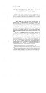


![Cost Optimization Pillar [PDF]](https://m.moam.info/img/260x300/cost-optimization-pillar-pdf_6479b31b098a9e2a3a8b457b.jpg)