the use of HI-MASS in the modeling and simulation ... HI-MASS is a C++ based system developed .... is easily modeled in HI-MASS by simply not send- ing a tp ...
A SIMULATION MODEL OF A SURVEILLANCE RADAR DATA PROCESSING SYSTEM USING HI-MASS Steven D. Farr Alex F. Sisti US Air Force Rome Laboratory 32 Hangar Road Gri�ss AFB, New York 13441, U.S.A.
ABSTRACT This paper discusses the model speci cation, construction of the executable model, model execution, and the simulation results of a simulation model of a surveillance radar data processing system that was developed using the Hierarchical Modeling and Simulation System (HI-MASS). HI-MASS is an object oriented C++ based system that supports model speci cation (modeling) using the Hierarchical Control Flow Graph Model paradigm and executes simulation models using the sequential synchronous simulation execution algorithm. Models speci ed in this model paradigm use two complementary hierarchical speci cation structures, one to specify the model components and their interconnections and the other to specify the behaviors of the individual components. The components and their interconnections are speci ed in HI-MASS via visual interactive modeling.
1 INTRODUCTION This paper is a companion paper to two other papers contained in these proceedings. One of these papers provides an overview of Hierarchical Control Flow Graph (HCFG) Models (Fritz and Sargent 1995; see Fritz and Sargent 1993 for additional information on HCFG Models) and the other paper provides an overview of the Hierarchical Modeling and Simulation System (HI-MASS) (Fritz, Sargent and Daum 1995; see Fritz, Daum, and Sargent 1995 for additional information on HI-MASS). HI-MASS uses the HCFG Model paradigm for model speci cation. It is assumed that a reader of this paper is familiar with these two papers. The primary purpose of this paper is to illustrate the use of HI-MASS in the modeling and simulation of a non-trivial system. The system we model and simulate is a surveillance radar data processing system. The purpose of this model is for performance
Douglas G. Fritz Robert G. Sargent Simulation Research Group Syracuse University 439 Link Hall Syracuse, New York 13244, U.S.A. evaluation studies. Hierarchical Control Flow Graph Models use two complementary types of hierarchical model speci cation structures. The rst type speci es the components that make up the model and how they are interconnected. This speci cation is called a Hierarchical Interconnection Graph (HIG). The second type of speci cation, the HCFG, is used to specify the behaviors of the individual atomic components of the model. HI-MASS is a C++ based system developed speci cally for Sun SPARC workstations running SunOS (Unix); however, HI-MASS has also been run on other systems which include an IBM RS/6000, a DEC Alpha, and Intel based personal computers. The system was developed by the Simulation Research Group at Syracuse University under contract to the U.S. Air Force's Rome Laboratory. HI-MASS provides a Graphical User Interface (GUI) for specifying the HIG using visual interactive modeling. HCFG speci cations are currently constructed via C++ code built upon a foundation of classes and functions supplied by HI-MASS. The remainder of the paper contains the following: an overview of the radar data processing system in Section 2, a description of the simulation model in Section 3, the simulation results in Section 4, and a summary in Section 5.
2 RADAR OVERVIEW The simulation model created was that of a data processing system similar to those used in recent vintage Air Force surveillance radar systems. The modeling of such a data processing system can aid in the design of a new system or in assessing the suitability of incorporating new CPUs into an existing system. A GPSS model of this system is described in Farr (1995). The radar data processing system is comprised primarily of four CPUs, global and local memories, I/O handlers, a display, a modem, and two buses.
Figure 1: Top Level Coupled Component Speci cation A separate CPU is used for radar control, signal processing, target processing, and communication. These processors handle messages and process data as appropriate to their functions. The primary function of the Radar Control (RC) processor is the handling of templates and target detection reports. This includes (1) the retrieving of templates for each radar beam from global memory and forwarding them to the Signal Processor (SP), and (2) the retrieving of target detection reports from SP for each radar elevation scan and forwarding them to global memory. The templates include information such as waveform and steering angles and are used to tailor the beam for each elevation scan; thereby, avoiding the presentation of returns from mountains, buildings, or other structures within range of the radar to the operator. Secondary functions for the RC processor include the creation and handling of diagnostic reports.
The Target data Processor (TP) is responsible for three major functions: (1) eliminating reports that have unlikely parameters and duplicate reports from adjacent beams, (2) estimating target altitude, and (3) storing the resultant reports in a Global Memorybased target table. All reports for a given scan are read into local memory and sorted by target range. The Communication (COMM) processor is tasked with sending data to the modem and display. The target data for each elevation scan is read into COMM's local memory and immediately sent to the display queue. However, the COMM modem processing is not straightforward because the modem queue may ll during greater than nominal conditions. If the target data cannot be placed into the modem queue, the report's reference is placed into a backup array internal to COMM. COMM later transfers the data to the modem queue as slots become available. In addition to the varied processing functions of the
Figure 2: Data Processor Coupled Component Speci cation CPUs, the data processing system handles messages and data of various lengths using two buses that have di�erent performance speci cations. The system also handles operator requests for background diagnostics and allows for the speci cation and use of new templates.
3 THE MODEL The HIG consists of the three coupled component speci cations (CCS's) shown in Figures 1, 2, and 3. They were developed via visual interactive modeling using the HI-MASS GUI. The top level CCS, shown in Figure 1, has two atomic components (indicated via a horizontal line near the top of the component box) and two coupled components. The CCS's for the data processor and output devices are shown in Figures 2 and 3, respectively. The HCFG Model paradigm allows for an arbitrary number of levels of
hierarchy in the HIG; however, we only use two levels in this model. In the top level CCS (Figure 1), both single channels and multichannels (bundles of channels) are used. The use of multichannels simpli es the speci cation of CCS's. Messages are used in this model to request and release resources. Note that there are no external ports in the top level CCS.
Figure 3: Output Devices Coupled Component Speci cation
The data processor coupled component shown in Figure 2 represents the four CPU's and the two buses as atomic components. In HI-MASS, connection boxes (represented by diamonds) are used to specify channel connections when multichannels split or merge and also to specify those connections that do not have a straightforward graphical representation. We have chosen, as shown in Figure 2, to use a separate connection box to connect each atomic component in Figure 1 to the atomic components in Figure 2; e.g., connection box 1 speci es the connections from the radar atomic component. By contrast, we could have used a single connection box to specify all interconnections within this CCS. However, the approach selected employs a direct mapping and results in less complexity within each connection box. We note in Figures 1, 2, and 3 that only single channels are used to connect the output devices coupled component. This was done to illustrate the use of single channels. One could have used a multichannel of size 2 and a corresponding connection box in the output devices CCS. Alternatively, the display and modem could have been speci ed as atomic components in Figure 1 and thus there would be no output devices coupled component. HI-MASS provides a software tool that maps the set of CCS's for a HIG into an Interconnection Graph. Information from the Interconnection Graph is used in constructing the simulation model. HI-MASS uses the sequential synchronous simulation execution algorithm, which requires that priorities be assigned to the atomic components. Examples of the priorities used are the highest priority was assigned to the bus1 atomic component and the lowest priority to the radar atomic component. An HCFG is required to describe the behavior of each type of atomic component used in the model. Each HCFG consists of a top level Macro Control State (MCS), and possibly child MCS's. (Recall that MCS's are encapsulated and thus they have their own name space.) The top level MCS for the TP processor is shown in Figure 4. This MCS contains eight (simple) control states and three child MCS's. The three child MCS's in Figure 4 are instances of the same type of MCS (shown in Figure 5), which demonstrates the reuse capability of MCS's. (While HCFG's allow any number of MCS levels in its hierarchy, the HCFG speci ed here for the TP uses only two levels of MCS's. HI-MASS also allows a modeler to replace the automatically generated numeric port identi ers with mnemonic port identi ers as was done between Figure 2 and Figures 4 and 5 for the TP atomic component.) The TP handles two priority levels of processes.
Target Report processing functions carry the highest priority and are capable of preempting the background diagnostic processing functions. There are two separate target report processes: one for each individual target report and one associated with each 30 millisecond elevation scan. TP also handles two types of background diagnostic processes: one for conducting its own diagnostics and one for producing a comprehensive diagnostic report once all the processors have completed their individual diagnostics. To explain part of the TP HCFG, let us assume that while the TP is idle (in control state S0 of the top level MCS), TP receives a request to perform background diagnostics. The message arrival on the bd request port causes the Point of Control (POC) (which always resides at the current control state) to move from S0 to S2. The TP will then remain in S2 until the 3 second background diagnostics is completed (as speci ed by the bd proc time() function) unless a message arrives on the rc done port indicating that a target report needs to be processed. Assume a message arrives on the rc done port prior to the completion of the diagnostic check. The arrival of this message causes the POC to leave S2 of the top level MCS and enter the preempt1 MCS (which is an instance of the TR Processing MCS type) via pin \in". When the target report processing has been completed by the preempt1 MCS, the POC leaves the preempt1 MCS via its \out" pin and returns to S2 of its parent MCS (which is TP's top level MCS). The TP then attempts to complete the diagnostic check. When the background diagnostic has been completed (requiring a total of 3 seconds), the POC moves from S2 to S0. The TR Processing MCS type depicted in Figure 5 manages the TP CPU time to process a target report and access the bus. When the POC enters the \in" pin it proceeds directly into the control state S0. It remains in S0 for 2 milliseconds which is the time speci ed by the tr proc time() time delay function for the TP to perform the report analysis. The POC then leaves S0 and enters S1 executing the event request bus1(). This event sends a message to bus1 requesting the use of bus1. The POC remains in S1 until a message is received from bus1 on port bus1 granted indicating that TP has use of bus1. The POC then leaves S1 and enters S2. The POC remains in S2 for 0.02 millisecond which is the time speci ed by the tr xfer time() time delay function. The POC then leaves S2, executes the event job1 complete(), and leaves this MCS via pin \out". (The POC then continues on to S2 of its parent MCS as described above.) Included in the execution of event job1 complete() is the sending of a message to bus1 indicating that TP
S0 process
tr_proc_time() request_bus1()
bus1_granted arrival_event()
S1 wait
S2 use_bus
in
tr_xfer_time() job1_complete() out
Figure 4: Target Processor (TP) Top Level MCS
1
S0 Idle 4
3
rc_done arrival_event()
(TR_Processing)
2 new_el_scan arrival_event()
in process1 out Figure 5: TR Processing MCS Type fixed_proc_time()
e_null() has nished using bus1. S1 bd_request One of TP's majorarrival_ functionsprocess2 is the identi cation comm_bd_done and removal of falseevent() targets from the system. Aparrival_event() proximately 12% of the targets will be marked as bd_proc_time() false because they are either duplicates of other tar2 job3_complete() S2 get reports orS3have unlikely parameters (i.e., unlikely process3 wait5 combinations of range, altitude and velocity). This TP is easily modeled in HI-MASS1 by simply not sendrc_done ing a tp done message 12% of the time to the COMM arrival_event() rc_bd_done (TR_Processing) mesatomic component. The sending of the tp done arrival_event() sage is handled by the job1 complete() inevent preempt1 in the MCS shown inS4Figure 5. The simulation model consists of 25 types of obwait6 jects: 10 atomic components (as shown2 incomp_proc_time() Figures request_bus1() S5 for each 1, 2, and 3), 10 top level MCS's (one atomic tp_bd_done process4 component), 4 sublevel MCS's, and the \Model". The arrival_event()
four sublevel MCS's consist of the MCS shown in Figure 5, a similar MCS for RC processing, a MCS for generating the completion of an elevation scan by the radar every 30 milliseconds, and a MCS to generate target report messages using an Erlang{2 distribution function for interarrival times. The \Model" contains a list of the atomic components which comprise the model and the port interconnection speci cation; both pieces of information are extracted from the Interconnection Graph. out Each type of object is de ned by a C++ class. All the C++ classes used were either comp_xfer_time() provided as part of job4_complete() HI-MASS or were constructed as classes derived from base classesbus1_granted provided as part of HI-MASS (e.g., class arrival_event() S6 S7 \Model", class \AC" (for atomic components), and wait4 \MCS"). Each class de nition use_bus4 class was compiled into
1 rc_done arrival_event() in
(TR_Processing) preempt2
out
object code. The object code was then linked with the HI-MASS and C++ libraries to form an executable model (program). To conduct simulation experiments, experimental frame les need to be speci ed for the executable model to use during its model construction and initialization phase. Speci c experimental frame les were constructed for each experiment.
4 SIMULATION RESULTS Two types of experiments were conducted | pilot runs and production runs. The pilot runs were a series of experiments conducted for the purpose of model veri cation and to perform a sensitivity analysis to identify the model parameters to be studied during the production runs. Model veri cation was accomplished by comparing simulation results to the anticipated, hand calculated, results and by comparison to the results produced by another model (Farr 1995) of the same radar data processing system. Both compared favorably. We present in Table 1 a sequence of messages extracted from the trace output generated by the simulation model to illustrate the sequence of messages that occur between the detection of a target by the radar and the presentation of that information on the operator display. (Table 1 uses the port identi er syntax de ned by HI-MASS. In HI-MASS the individual ports of a port array that are created by multichannels are identi ed using a zero based index. For example, bus2.3[1] is the port identi er for the second element of the input port array \3" of atomic component bus2 shown in Figure 2.) The passage of time is not shown in the table and occurs between the generation of messages. In one experiment, the model was executed with a simulation time of 6 seconds corresponding to one revolution of the radar and with a target interarrival time speci ed such that the system is working at its peak loading of 1600 targets. Using a Sun SPARC2 equivalent, the simulation took approximately 55 seconds of \wall clock" time during which 1565 targets were simulated and 26,427 messages were generated within the model. HI-MASS produces an end of simulation output that identi es the state of each object at the time the simulation terminates. Because the code for the HIMASS model is completely accessible, the user has the option to customize the output data stream as the simulation progresses. Shown in Table 2 is a portion of the end of simulation output for the radar atomic component. In this case, the simulation time for the
Table 1: Target Report Message Sequence From: OutPort To: InPort radar.1[0] SP.2
Comment target detected
SP.1[0]
RC.1[0]
end SP
bus2.3[0] RC.5 bus2.3[1] bus1.2[0] RC.7 bus1.2[1] TP.1[0]
bus2 requested bus2 granted bus2 released bus1 requested bus1 granted bus1 released end RC
bus1.4[0] TP.6 bus1.4[1] COMM.1[0]
bus1 requested bus1 granted bus1 released end TP
bus1.6[0] COMM.5 bus1.6[1] display.1
bus1 requested bus1 granted bus1 released end COMM
SP
Target Report Processing
RC
Target Report Processing
TP
Target Report Processing
RC.4[0] bus2.4 RC.4[1] RC.8[0] bus1.1 RC.8[1] RC.2[0] TP.7[0] bus1.3 TP.7[1] TP.2[0]
COMM
COMM.6[0] bus1.5 COMM.6[1] COMM.7
Target Report Processing
experiment was set to 300 milliseconds. Table 2 shows that when the simulation terminated, the POC for the radar atomic component was at control state s0 of the delay1 (type Erlang{2 Delay) child MCS contained within the top level MCS (of the radar atomic component). It also shows that the value of the radar's local simulation clock was 296.397 and its next event was scheduled for time 302.957. These three pieces of information are automatically generated by HI-MASS for each atomic component in the model. Additional model and/or experimental frame speci c end of simulation output may be speci ed by the modeler. An example of model speci c output is the number of messages sent by the radar during the course of the simulation run, i.e., msgCount == 79. Table 2: Sample End of Simulation Output AC::EofSim_local_dump() - "radar(Radar)" clock_ = 296.397 nextEventTime_ = 302.957 current_ ="radar(Radar)::/top/delay1(E2Delay)::s0" mean_ == 3.75 el_scan_ == 30 MCS::EofSim_local_dump() - "radar(Radar)::/top(Radar)" msgCount_ == 79
HI-MASS simulationtime, initial component states, and other input parameters (e.g., mean and el scan ) are set using the experimental frame which allows the user to vary these parameters without having to modify the C++ source code, recompile the changes, and relink between experiments.
5 SUMMARY HI-MASS o�ers an extremely exible way to perform discrete event simulation. The hierarchical nature of the HCFG Model paradigm allows for the representation of complex systems in such a way that is intuitive and comprehensible. Working at the component level o�ers a means to build models that are highly modular in nature; thus, o�ering modelers the bene ts that have been associated with modular programming techniques. We found that modeling atomic component behaviors using HCFG's, which favors the use of the active resource process world view (as contrasted to the active transaction process world view), worked extremely well. The speci cation of CCS's for the HIG via visual interactive modeling in HI-MASS was easy. The speci cations of the HCFG's via MCS's for atomic components required an understanding of the classes and functions provided by HI-MASS and a working knowledge of C++ program development in a Unix based environment. These speci cations were straightforward and not di�cult. Running a HI-MASS model was simple.
REFERENCES Farr, S.D. 1995. Simulation of Surveillance Radar using GPSS/H Rome Laboratory Technical Memorandum RL-TM-xx. Fritz D.G. and R.G. Sargent. 1993. Hierarchical Control Flow Graphs. Case Center Technical Report 9323, Syracuse University. Fritz D.G. and R.G. Sargent. 1995. An Overview of Hierarchical Control Flow Graph Models, In Pro-
ceedings of the 1995 Winter Simulation Conference.
Fritz, D.G., R.G. Sargent, and T. Daum. 1995. An Overview of HI-MASS (Hierarchical Modeling and Simulation System), In Proceedings of the 1995 Winter Simulation Conference. Fritz, D.G., T. Daum, and R.G. Sargent. 1995. User's Manual for HI-MASS, Simulation Research Group, 439 Link Hall, Syracuse University.
AUTHOR BIOGRAPHIES STEVEN D. FARR is an electronics engin-
eer at the US Air Force's Rome Laboratory (http://www.rl.af.mil). Steve received his B.S. from the University of Connecticut in 1983, a MBA from Rensselaer Polytechnic Institute in 1986 and a M.S. from Syracuse University in 1993. His professional responsibilities include the application of emerging technologies to speci c modeling and simulation requirements.
ALEX F. SISTI is an Electronics Engineer with the Intelligence Technology Branch, Signals Intelligence Division, the Intelligence and Reconnaissance Directorate at Rome Laboratory, Gri�ss AFB, NY. He has been actively applying his modeling and simulation research interests in a variety of Air Force programs over the last 10 years. He received an A.A.S. degree in Accounting in 1975, a B.S. in Computer Science in 1982 and earned his M.S. in Computer Engineering from Syracuse University in 1989. DOUGLAS G. FRITZ is a graduate student
at Syracuse University working towards a Ph.D. in Computer Engineering. His research area is hierarchical modeling for discrete event simulation. He received M.S. degrees in Electrical Engineering and Computer Science from Syracuse University and a B.S. degree in Electrical Engineering from The Pennsylvania State University. He was formerly with IBM as a development engineer for high speed switching systems.
ROBERT G. SARGENT is a Professor at Syra-
cuse University. He received his education at the University of Michigan and has published widely. Dr. Sargent has served his profession in numerous ways and has been awarded the TIMS College on Simulation Distinguished Service Award for long-standing exceptional service to the simulation community. His research interests include the methodology areas of modeling and discrete event simulation, model validation, and performance evaluation. Professor Sargent is listed in Who's Who in America.