interest in simulation modeling for ERP systems, as well as my academic interest
... decided to develop a simulation prototype for an ERP application.
A simulator prototype for an ERP system Oscar Alfonso Caceres Mendoza
LYNGBY 2005 MASTER THESIS PROJECT NR. 2005/87
══════
IMM ══════
2
Preface This Master Thesis was carried in order to fulfill the curriculum for the M.Sc.. in Computing and Mathematics program at the IMM department in the summer of 2005. Working on this project has been a challenging and educational experience, all the more so because its conception and application are both based on my professional interest in simulation modeling for ERP systems, as well as my academic interest in computing and mathematics. I would like to express my sincere gratitude to Bo Friis Nielsen from IMM-DTU for his invaluable guidance and support during my time on this project.
3
Abstract The following document presents an investigation based on the idea of improving the value of Enterprise Resource Planning (ERP) systems by adding a discrete event simulation application to the ERP framework. First, I conducted a brief investigation to assess whether discrete event simulation is already included in most (or any) ERP applications. I found that this type of simulation is not common to ERP systems, and is particularly lacking in systems designed for small- and mid-sized organizations. Perceiving an opportunity to enhance the functionality of existing ERP systems, I decided to develop a simulation prototype for an ERP application. This project is the subject of my Master thesis. To achieve the goal of developing a simulation tool, I conducted research on the structural and functional requirements for my prototype, placing emphasis on ease of use and the interaction between the data-fitting and modeling phases of simulation. I chose to develop this simulation prototype for The Microsoft Navision ERP software solution, with which I have several years of experience as a software developer. In the course of developing the prototype, I found that Navision lacked certain desired functions for performing statistical operations and designing graphical models. I solved this problem by creating external components that can be used within the Navision development environment. Basic testing was performed in order to provide reasonable assurance that the external components would function correctly. In the end, my efforts to develop simulation capabilities within the Navision ERP system proved successful. As often occurs during the development process, I was inspired to create new functionality that I had not included in my original requirements. I attribute this creative inspiration, in part, to the wide scope of simulation modeling as a concept. I found that my simulation prototype has the potential to add value to many areas of the modular and integrated framework of an ERP system for a result that is greater than the sum of its parts.
4
In conclusion, I believe that simulation modeling can add significant value to existing ERP systems, and that future research should be done in order to automate the data analysis process so as to enhance the adoption of simulation techniques for the current users of ERP applications.
5
Table of Contents Table of Contents ..................................................................................................... 5 Introduction.............................................................................................................. 7 PART I: Concepts and Definitions.......................................................................... 9 1. ERP Systems......................................................................................................... 9 1.1.
What is an ERP system?....................................................................................9
1.2.
Simulation on ERP software ...........................................................................10
1.3.
Microsoft Navision ...........................................................................................12
1.3.1. 1.3.2.
Microsoft Navision Development environment.........................................................14 History of Microsoft Navision - former Navision A/S ..............................................15
2. Simulation .......................................................................................................... 17 2.1. 2.1.1.
Definition...........................................................................................................17 Simulation concepts ...................................................................................................17
2.2.
The modeling process.......................................................................................19
2.3.
When to use simulation....................................................................................21
2.4.
Stochastic processes in simulation ..................................................................22
PART II System Design ......................................................................................... 31 3. Conceptual Design ............................................................................................. 31 3.1.
Data Analysis ....................................................................................................34
3.2.
Simulator...........................................................................................................37
3.2.1. 3.2.2.
3.3.
Drawing Tool.............................................................................................................37 Simulation Execution.................................................................................................47
Summary...........................................................................................................53
4. Logical Design.................................................................................................... 55 4.1. 4.1.1. 4.1.2.
4.2. 4.2.1. 4.2.2.
NaviMath and NaviSim automation servers..................................................56 NaviMath.dll ..............................................................................................................57 NaviSim.dll ................................................................................................................59
Navision Objects...............................................................................................65 Data Fitting ................................................................................................................69 Simulation Model Creation........................................................................................90
6
4.2.3.
Simulation Model Execution .....................................................................................97
PART III Implementation and Testing ............................................................... 108 5. Implementation ................................................................................................ 108 5.1.
Implementation Plan......................................................................................108
5.2.
NaviMath.dll...................................................................................................109
5.2.1. 5.2.2. 5.2.3.
5.3. 5.3.1. 5.3.2. 5.3.3. 5.3.4.
5.4. 5.4.1. 5.4.2. 5.4.3. 5.4.4.
INaviMath Interface.................................................................................................109 NaviMath Class........................................................................................................110 RandomGen Class....................................................................................................112
Data Fitting.....................................................................................................113 Creation of Temp Data Table...................................................................................113 Kolmogorov-Smirnov Test ......................................................................................117 Chi-Square Test .......................................................................................................119 Creation of Frequency table.....................................................................................122
Simulation Execution.....................................................................................123 Engine ......................................................................................................................123 Next Event Method ..................................................................................................126 Joiner implementation..............................................................................................128 Router Implementation ............................................................................................129
6. Testing .............................................................................................................. 132 6.1. 6.1.1.
6.2.
Data Fitting.....................................................................................................132 Goodness-of-fit tests ................................................................................................136
Simulation Execution.....................................................................................137
7. Conclusions ...................................................................................................... 139 7.3.
Future Work...................................................................................................142
Appendix A Script for creating Interval Data..................................................... 144 Appendix B Exponential data used for testing the goodness-of-fit tests............ 145 Appendix C Simple 1 model log........................................................................... 146 Appendix D Simple 2 model log........................................................................... 148 Appendix E Joiner Test model log....................................................................... 151 Appendix F Router Test model log...................................................................... 155 Appendix G Test Script for the Router Shape..................................................... 159 References ............................................................................................................ 162
7
Introduction Since the introduction of Material Requirement Planning (MRP) systems in the 1960s, Management Information Systems (MIS) have enjoyed a steady growth and have become an essential tool for managing the operations of a company. Originally aimed at manufacturing companies and large corporations, MRP grew into Enterprise Resource Planning (ERP) – which is itself now a dated acronym. ERP systems are currently used in all the Fortune 500 companies, a market that in 2003 was worth a staggering sum of 61 billion dollars. In both my first job and my current position of employment, I am involved in the development of ERP software for small- and mid-size businesses. Each year, we learn of new requirements and technologies that make this market an interesting and challenging and attractive space in which to compete. The main goal of ERP software is to act as the central interaction point of different areas of an organization in order to facilitate sound, informed decision-making about operations. In effect, the ERP system becomes the main repository for the company’s data. This centralized approach suggests and inspires a variety of applications, such as handheld applications that retrieve and update data from and into the main system; e-commerce applications, human workflow, e-billing and eprocurement. Simulation modeling is another tool designed to aid the decision-making process. A simulation takes input data and processes that data against a model or template that represents a simplification of a certain reality or situation. There exists an observable relationship between the concepts or ERP and simulation modeling that, in my opinion, is underutilized and worthy of serious academic investigation. Although I have worked for an ERP software vendor for more than five years, I have never heard the concept of simulation modeling applied in that context. It is my belief that simulation modeling software could become an indispensable tool for ERP and other areas of business operations. The very thought of being able to simulate various elements of a company’s operation, observe the probable outcomes of predefined scenarios, and make decisions accordingly is a managers dream.
8
All these ideas were the foundation to what is now presented to you as a Masters Thesis project. With this project I would like to answer some questions concerning the use of simulation software in ERP systems. Some of these questions are: -
Is simulation used in some ERP systems today? If so, in what areas? Is it possible to create a simulation module in the ERP system that I have been working for? If possible, What would this system need? What functionality could it have and how could it use the potential that is already part of the ERP software. What do I think can be done to enhance the simulation application developed?
The answers to the questions concerning the possibility of including a simulation application in an ERP system would be obtained by developing a simulation prototype for the Navision application. Navision is the ERP system were I have had all my working experience and is an application that is used by small and medium size companies. This market is very large and makes it the perfect environment to test the usability of simulation software for average users that do not have extensive knowledge of mathematics or statistics. This document is partitioned in four parts. Part I describes introductory concepts related to simulation in ERP systems, the history of the Navision and ERP systems in general, simulation and related concepts that would be use on the project. Part II describes the ideas and the design of the proposed simulation prototype system. Part III describes the implemented parts of the design, how were they tested and what conclusions were found in this project. Potential areas of research and thoughts in regards to the future of simulation in the ERP market are also given.
9
PART I: Concepts and Definitions This section briefly describes the basic concepts and definitions that are going to be used through out this document.
1. ERP Systems 1.1.
What is an ERP system?
The contents of the chapter are a summary of the concepts found in the Enterprise Resource Planning definition in the Wikipedia encyclopedia [11]. Enterprise resource planning systems are management information systems that integrate and automate many of the business practices associated with the operations or production aspects of a company. Enterprise resource planning is a term derived from material resource planning. ERP systems typically handle the manufacturing, logistics, distribution, inventory, shipping, invoicing and accounting for a company. Enterprise Resource Planning or ERP software can aid in the control of many business activities, such as, sales, delivery, billing, production, inventory management, and human resources management. ERPs are cross-functional and span the entire enterprise wide. All functional departments that are involved in operations or production have their functions integrated in one system. In addition to manufacturing, warehousing, and shipping, this integration also includes: accounting, human resources, marketing, and strategic management. To implement ERP systems, companies often seek the help of an ERP vendor or of third-party consulting companies. Consulting in ERP operates on two levels: business consulting and technical consulting. A business consultant studies an organization's current business processes and matches them to the corresponding processes in the ERP system, thus 'configuring' the ERP system to the
10
organisation's needs. Technical consulting often involves programming. Most ERP vendors allow changing their software to suit the business needs of their customer.
1.2.
Simulation on ERP software
In order to have an overview of the existence of simulation software in the ERP industry a small investigation was conducted. This investigation consisted in searching the offerings concerning simulation of all the big players of the ERP arena. The result of this research is presented in the following table: Vendor SAP [5]
Oracle (PeopleSoft and J.D. Edwards) [14]
Microsoft Business division[12]
Solutions
Has a Simulation software? Yes, but in a different degree. The modules is called Business Intelligence and has a modules called BPS, business planning and simulation. It is mainly oriented to be used for planning of projects and people involved and run simuilations on expected results on the project. Workforce simulation. Use to simulate different scenarios regarding compensations and budgeting. Traffic simulation based on radio frequency.
Limited offering
The Sage Group[13]
No offering
SSA Global Technologies (which acquired Baan) [6]
Manufacturing scheduling. A simulator for manufacturing scenarios. Yes, but focused on the manufacturing area. A part of the Movex module. Can
Intentia International AB)[4]
Similar products Powersim, add on product that is not part of the basic offering but that it uses the BPS engine.
Includes business execution process manager language, a tool for modeling business processes that is aim at integrating services. In other words a service orchestration tool [15] Human workflow solution. Based on notifying user on events that occur on the system. The workflow engine can be use for creating a simulation model. Simulation for quotes prices based on different material configurations
11
be used to simulate different scenarios concerning the manufacturing or maintenance strategies.
Table 1 Simulation in ERP software
As it can be seen from table 1, many large software vendors do include simulation in their current offering. However, there are a few, if any, global or generic simulation application that can be used for any user-defined areas (the focus is mostly in the areas of supply chain and finance). Most of the simulation capabilities in theses products do not relate to discrete event simulation and is more closely linked to impact analysis tools based on different data configurations. For this reason, it is possible to say that the use of a generic discrete event simulation application to be included in an ERP system it is, upon first glance, an unexplored area of opportunity. With these points in mind, the aim of this project is to design and develop a simulator prototype for an ERP system, more precisely, the Navision software package. It is important to clarify that there is a plethora of simulation applications available in the software market e.g. Arena, GoldSim, Simul8. However, all of them are stand-alone applications that offer integration capabilities with other systems and are not included in ERP systems.
12
1.3.
Microsoft Navision
Microsoft Navision is a well-established ERP solution aimed at the smaller end of the market and is particularly suited to wholesale distribution and manufacturing. One key area where Navision adds value is in a ‘hub-and-spoke’ environment, where Navision is used at the ‘spokes’ and reports to a central HQ solution. Customers are typically small- and medium-sized organisations, with 1-50 users, and the largest customer base is in the core industry sectors of wholesale distribution, manufacturing, and services. Microsoft Navision is delivered to customers in modular packets known as ‘granules’. This feature of Navision enables customers to select the specific components of the Navision system that they require, with the freedom to add extra granules over time as the needs of the business change. All modules are based around a core financials application, with a user-based pricing model that enables customers to pay only for what they use. The core Navision functions provide a scope of coverage that is typical of ERP solutions–financial accounting, inventory management, supply-chain management, transaction tracking and auditing, as well as management systems for other company resources such as personnel. However, Navision also supports functional areas that are not traditionally part of ERP, such as professional services, business analytics, and e-business infrastructure. Microsoft Navision Version 4.0 provides a fuller level of integration with the Microsoft family of software products. The user interface has a new look and feel that takes its cue from Microsoft Outlook, and integrations with Microsoft Word and Excel have been improved, especially for reporting functions. The latest version of Navision also has sophisticated analytics capability, which allows small businesses to achieve the level of visibility into underlying data, including predefined yet flexible Key Performance Indicators. In addition, Navision 4.0 introduces the concept of business notification–a workflow technique designed to improve productivity and collaboration by alerting users to important issues that pertain to their role in the business. For example, if a sales margin is particularly low. Navision uses a technique called Sum Index Flow
13
Technology (SIFT) to enable consolidation of data based on user-defined dimensions, which can be easily changed. SIFT is a proprietary method for rapidly recalculating totals as data flows into the system. This method enables the user to run queries at a range of different levels; for example, monthly or yearly. Navision can be deployed on an Intel platform running Microsoft Windows 2000 or Windows XP. Navision uses Active Directory for directory services on distributed networking environments and stores information on primary settings for users. The underlying database can be either the proprietary C/SIDE database or Microsoft SQL Server. In cases where OLAP-querying capabilities are required, the SQL Server database is necessary. Deployment is usually carried out by the Microsoft Business Solutions partner, in conjunction with a team from the customer organisation. After deployment, limited resources are likely to be needed for maintenance and administration, and these are usually provided by the customer themselves. Navision is known for its ability to be rapidly implemented, and Microsoft Business Solutions now provides templates and a methodology to help partners implement the Navision system as quickly and efficiently as possible. As one would expect from an ERP system, integration with third-party applications is possible and can be carried out using different technologies, including XML, ODBC. Navision is tightly integrated with Microsoft’s technology stack, including Microsoft BizTalk Server, Word, and Outlook (for integration between Outlook contacts and Navision). While the ‘sweet spot’ for Navision is between 20 and 45 concurrent users, the company states that the solution can be scaled upwards, although it is not appropriate for hundreds of users. The C/SIDE database is very robust and includes a ‘version principle’ that allows reports to be generated without locking other users out of the database. Each time a transaction is committed, a new version of the database is created. This function enables employees and applications to access and modify the system concurrently and provides a failsafe against catastrophic power failure.
14
1.3.1. Microsoft Navision Development environment C/SIDE (Client Server Integrated Development Environment) is the environment in which it is possible for developing applications for the Navision product. A C/SIDE application is composed from seven types of application objects. Each type of application object is created using a specific tool called a designer. The application objects you create using these designers are all based on some general concepts. A fundamental knowledge of these concepts speeds up the C/SIDE application development process. There are seven basic objects in C/SIDE: The table, form, report, dataport, codeunit, xmlport and the menusuite objects. The Table object is used to describe how data will be stored in the database and how it will be retrieved. The Form object is used to display data to the user in a familiar and useful way. Most forms allow the user to add records to a table, view and modify records as well. The Report object enables the user to summarize and print out detail information using the filters and sorting that he or she chooses. The Dataport object allows the user to export or import table data. The Codeunit object allows that work with Navision to organize and group the code that they write. enables automated XMLbased communication ‘agents’ to harvest and transform table data. XMLport is used primarily in conjunction with some communication component as a means of integrating with third-party applications. Finally, the Menusuite object allows the creation of custom menus that can be used to group functionality in common areas. C/SIDE is not object-oriented, but rather it is object-based. This is an important distinction to note. In an object-oriented language or environment, the developer can create new types of objects based on the ones already in the system. In C/SIDE, you have only the seven fore-mentioned types of application objects to choose from. While this feature limits Navision in a certain respect, it is intended to optimize the speed and performance factor of C/SIDE. Navision is also optimized in this manner to simplify and streamline development, allowing coders and engineers to work with greater speed and efficiency while reducing the risk of severe bugs and defects.
15
C/AL is the language that the C/SIDE application compiles and run. This language is based significantly on the PASCAL computer language and is very intuitive and easy to learn.
1.3.2. History of Microsoft Navision - former Navision A/S The following section is an extract from the Software Advisor web site [10] where the history of Navision is described. Navision was originally founded in 1983 by Jesper Balser, Peter Bang and Torben Wind in Copenhagen, Denmark. In 1984 the product was launch as “PCPlus” in Denmark & Norway. This was a character-based accounting solution targeted towards the SOHO (small office/home office) market. In 1984 “Beauty of Simplicity” was adopted as the first company slogan. In 1987 the company changed its name to Navision and the product was renamed to Navigator. In 1990 the company launched Navision 3.0, and expanded the market beyond Scandinavia into Germany, Spain and the United Kingdom. In 1992, the company also reached an agreement to distribute Navision in the United States. In 1993 Navision initiated a major development effort to create a new generation of Navision solutions based on the Microsoft Windows 32-bit client/server platform. The company continued to enhance the product by adding contact management functionality in 1997, manufacturing capabilities in 1998, and advanced distribution in 1999. 2000 was a stellar year for Navision. In 2000 Navision Financials received Microsoft Windows 2000 Professional Certification and Microsoft Windows 2000 Server Certification. The company launched the Navision Commerce Gateway – world’s first solution based on Microsoft’s BizTalk Server. The company also launched the Navision User Portal – the world’s first solution based on Microsoft’s Digital Dashboard. In an industry shaking move, Navision Software merged with their long-time Danish rival Damgaard Software. In 2001 the company made many enhancements including: 1. Re-branded “Navision Financials” as “Navision Attain” and “Damgaard Axapta” as “Navision Axapta”; 2. Integrated the e-commerce applications, Commerce Gateway, Commerce Portal into both products; 3. Introduced User Portal, browser-based access to both products;
16
4. Introduced supply chain collaboration functionality, manufacturing and distribution capabilities, and new financial management functionality; 5. Navision received the Designed for Microsoft XP logo. In 2002 Microsoft acquired Navision for $1.4 billion – the largest acquisition ever made by Microsoft. Today Navision has been the fastest growing accounting system solution offered by Microsoft. Since then, the Navision software product line has grown steadily and today has approximately 35,000 customers worldwide, and more than 400,000 individual users. The Navision product’s strength and future outlook has never looked stronger. Navision is mainly targeted to mid market companies located in the mid-low end of the market. The typical Navision user is a company with around 70 to 100 employees per location and sometimes is part of a bigger conglomerate. This market is characterized by a focus on solving day to day operations and requires fast and ease to understand solutions.
17
2. Simulation This chapter describes the simulation concepts and definition that would be use throughout the document. The contents of this chapter are a summary of the descriptions found in Banks and Carson [1] and Law and Kelton [2].
2.1.
Definition
Simulation is the imitation of the operation of a real-world process or system over time. Simulation involves the generation of an artificial history of the system, and the observation of that artificial history to draw inferences concerning the operating characteristics of the real system that is represented. Simulation is an indispensable problem-solving methodology for the solution of many real-world problems. Simulation is used to describe and analyze the behaviour of a system, ask "what if" questions about the real system, and aid in the design of real systems. Both existing and conceptual systems can be modelled with simulation.
2.1.1. Simulation concepts There are several concepts underlying simulation. These include: Model: A model is a representation of an actual system. Immediately, there is a concern about the limits or boundaries of the model that supposedly represent the system. The model should be complex enough to answer the questions raised, but not too complex as explained in the section above. Events: Consider an event as an occurrence that changes the state of the system. As an example, events include the arrival of a customer for service at the bank, the beginning of service for a customer, and the completion of a service. There are both internal and external events, also called endogenous and exogenous events, respectively. For example, an endogenous event in the example is the beginning of service of the customer since that is within the system being simulated. An exogenous event is the arrival of a customer for service since that occurrence is outside of the simulation.
18
System State Variables: The system state variables define what is happening within the system to a sufficient level at a given point in time. The determination of system state variables is a function of the purposes of the investigation, so what may be the system state variables in one case may not be the same in another case even though the physical system is the same. Entities and Attributes: An entity represents an object that requires explicit definition. An entity can be dynamic in that it "moves" through the system, or it can be static in that it serves other entities. For instance, a customer in a supermarket queue is a dynamic entity, whereas the cashier teller is a static entity. An entity may have attributes that pertain to that entity alone. Thus, attributes should be considered as local values e.g. the time of arrival, colour, shape, etc. This can be later used to differentiate the data and collect statistics accordingly. Resources: A resource is an entity that provides service to dynamic entities. The resource can serve one or more dynamic entities at the same time. These entities can request one or more units of a resource. If denied, the requesting entity joins a queue, or takes some other action (i.e., diverted to another resource, ejected from the system). If permitted to capture the resource, the entity remains for a time, then releases the resource. There could be many possible states of the resource e.g. idle and busy (minimal case), failed, blocked, or starved. List Processing: Entities are managed by allocating them to resources that provide service, by attaching them to event notices thereby suspending their activity into the future, or by placing them into an ordered list. Lists are used to represent queues. Lists are often processed according to FIFO (first-in-first-out), but there are many other possibilities. Activities: An activity whose duration is known before the activity begins. Thus, when the activity starts, its end can be scheduled. The duration of an activity can be a constant, a random value from a statistical distribution, the result of an equation, input from a file, or computed based on the event state. Delays: A delay is an indefinite duration that is caused by some combination of system conditions. When an entity joins a queue for a resource, the time that it will remain in the queue may be unknown initially since that time may depend on other events that may occur.
19
Discrete event simulation After defining relevant concepts of simulation modelling we are now able to introduce the concept of discrete event simulation. This type of simulation is the one that offers most interesting aspects to the author in relation with ERP systems and would be the focus of the project. A discrete-event model attempts to represent the components of a system and their interactions to such an extent that the objectives of the study are met. These models include a detailed representation of the actual internals of the system and are conducted over time (run) by a mechanism that moves simulated time forward. The system state is updated at each event along with capturing and freeing of resources that may occur at that time. State variables change only at those discrete points in time at which events occur. Events occur as a consequence of activity times and delays. Entities may compete for system resources, possibly joining queues while waiting for an available resource. Activity and delay times may hold entities for durations of time.
2.2.
The modeling process
The application of simulation involves specific steps in order for the simulation study to be successful. Regardless of the type of problem and the objective of the study, the process by which the simulation is performed remains constant. The following briefly describes the basic steps in the simulation process: 1. Problem Definition: The initial step involves defining the goals of the study and what needs to be solved. The problem is further defined through objective observations of the process to be studied. Care should be taken to determine if simulation is the appropriate tool for the problem under investigation (more clarification on this topic in the next section). 2. Project Planning: The tasks for completing the project are broken down into work packages with a responsible party assigned to each package. Milestones are indicated for tracking progress. This schedule is necessary to determine if sufficient time and resources are available for completion. 3. System Definition: This step involves identifying the system components to be modelled and the performance measures to be analyzed. Often the
20
4.
5.
6.
7.
8.
9.
system is very complex, thus defining the system requires an experienced modeller who can find the appropriate level of detail and flexibility. Model Formulation: Understanding how the actual system behaves and determining the basic requirements are necessary in developing the right model. Creating a flow chart of how the system operates facilitates the understanding of what variables are involved and how these variables interact. Input Data Collection and Analysis: After formulating the model, the type of data to collect is determined. New data is collected and/or existing data is gathered. Data is fitted to theoretical distributions. For example, the arrival times of a specific part to the manufacturing plant may follow an exponential distribution curve. Model Translation: The model is translated into programming language. Choices range from general purpose languages such as Fortran or simulation programs such as Arena. Verification and Validation: Verification is the process of ensuring that the model behaves as intended, usually by debugging or through animation. Verification is necessary but not sufficient for validation that is a model may be verified but not valid. Validation ensures that no significant difference exists between the model and the real system and that the model reflects reality in an acceptable way. Validation can be achieved through statistical analysis. Additionally, face validity may be obtained by having the model reviewed and supported by an expert. Experimentation and Analysis: Experimentation involves developing the alternative model(s), executing the simulation runs, and statistically comparing the alternative(s) system performance with that of the real system. Documentation and Implementation: Documentation consists of the written report and/or presentation. The results and implications of the study are discussed. The best course of action is identified, recommended, and justified.
21
2.3.
When to use simulation
Although knowing the basic steps in the simulation study is important, it is equally important to realize that not every problem should be solved using simulation. When simulation is applied inappropriately, the study will not produce meaningful results. The failure to achieve the desired goals of the simulation study is, many times, caused by the inappropriate application of simulation. To recognize if simulation is the correct approach, four items should be evaluated before deciding to conduct the study: 1. 2. 3. 4.
Type of Problem Availability of Resources Costs Availability of Data
Type of Problem: If a problem can be solved by common sense or analytically, the use of simulation is unnecessary. Additionally, using algorithms and mathematical equations may be faster and less expensive than simulating. Also, if the problem can be solved by performing direct experiments on the system to be evaluated, then conducting direct experiments may be more desirable than simulating. The real system itself plays another factor in deciding to simulate. If the system is too complex, cannot be defined, and not understandable then simulation will not produce meaningful results. This situation often occurs when human behaviour is involved. Availability of Resources: People and time are the determining resources for conducting a simulation study. An experienced analyst is the most important resource since such a person has the ability and experience to determine both the model's appropriate level of detail and how to verify and validate the model. Without a trained simulator, the wrong model may be developed which produces unreliable results. The schedule should allow enough time for the implementation of any necessary changes and for verification and validation to take place if the results are to be meaningful. Costs: Cost considerations should be given for each step in the simulation process, purchasing simulation software if not already available, and computer resources. Obviously if these costs exceed the potential savings in altering the current system, then simulation should not be pursued.
22
Availability of Data: The necessary data should be identified and located, and if the data does not exist, then the data should be collectible. If the data does not exist and cannot be collected, then continuing with the simulation study will eventually yield unreliable and useless results. The simulation output cannot be compared to the real system's performance, which is vital for verifying and validating the model.
2.4.
Stochastic processes in simulation
In order to model reality many simulation models include the use of random components. These components take the form of random numbers that follow a specific distribution (previously obtain in the data analysis process). In order to generate these distributions there are several methods that are base on random number generators. As mentioned in section 1.2 the main objective of this project is to build a simulation prototype that will reside inside the Navision application. Therefore, an important decision to make is to find out the distributions that would be more relevant for a typical Navision user. To aid the decision process the following considerations have been specified based on the needs of these users: a) There should be appropriate distributions to use when there is not enough data or only assumptions of the behavior of the data. In many occasions the user would not have the data needed in the system to estimate a distribution for it, hence the need for distributions that can be used with some assumptions about some plausible ranges. b) There should be a distribution that is suited when there is an abundance of data but is not desire to do a perfect fit or complicated calculations and formulas to model that behavior. Sometimes, obtaining the best distribution for a set of data is a demanding task in terms of experience and knowledge. In this case it should be possible to find a good approximation so the Navision users could still obtain satisfactory results. c) There should be a distribution suited for arrival and waiting processes. Arrival and waiting process would be, in my opinion, the most common modeling cases that a user would encounter. With this process types it can be possible to model, arrival of customers, service, sales, purchase documents, waiting time for machinery,
23
work performed by an employee, machine failures, to name but a few examples.
With the above considerations in mind the following distributions have been chosen: Considerati on Index a)
Distribution Name Uniform
Triangular
Explanation With this function the user can give a range of values when there is absence of data. With this function the user can give a maximum, minimum and most likely value when there is absence of data.
Algorithm to generate the distribution U(a,b): 1.- Generate U=U(0,1) 2.- Return X = a + (b-a)*U triang(a,b,c) 1.- Generate U=U(0,1) 2.- c´ = (c-a)/(b-a) 2.- if U ≤ c´, then X =
c´U
. Otherwise,
X= b)
Normal
Besides the fact that many data sets can be normally distributed. Because of the central limit theorem[7][8] this distribution can be applied to wide variety of cases in the presence of an average and variance in the observations.
(1 − c´)(1 − U ) .
3.- Return X´ = a + (b-a)*X N(µ,σ2) 1.- Generate U1=U(0,1) and U2=U(0,1) 2.X1=
− 2 ln U 1 * cos 2πU 2 3.X2=
− 2 ln U 1 * sin 2πU 2
c)
Exponential
Weibull
A very good and widely used distribution for arrival processes. It can be also used instead of a Poisson process too, since the inter-arrival time is exponentially distributed. It is widely used to simulate failures and waiting times. Also is a versatile distribution that can take the characteristics of other types of distributions.[9]
4.- return X´1= µ + σ*X1 5.- return X´2= µ + σ*X2 Exp(β) 1.- Generate U=U(0,1) 2.- Return X = - β lnU
Weibull(α,β) 1.- Generate U=U(0,1) 2.- Return X = β(-lnU)1/α
Table 2 Considerations for chosen distributions and algorithms to generate random variates.
24
The above mentioned distributions would also be use on the data analysis process since they are the only ones that the user would be able to use on the prototype. The reader should notice the omission of discrete distributions such as: Poisson, Geometrical and Binomial. These distributions are commonly used to quantify the number of entities arriving in a fix interval of time and estimation of success or failure events respectively. This kind of events will not be in the scope of the prototype. A fundamental part of the data analysis process is the goodness-of-fit tests that are going to be used. The most common ones to use are the Kolmogorov-Smirnov(KS) and Chi-Square tests, which would be prefer choice in this prototype. It is worth mentioning that there are other methods available but they are mostly heuristic ones that are not going to be implemented. Some of these methods are: histograms, box plots and probability plots. The goodness-of-fit tests are based on the null hypothesis (Ho) of no significant difference between the sample and the theoretical distributions. The major shortcoming that they present is that they are not very powerful for small to moderate sample sizes since they are not very sensitive for small disagreements between the data and the fitted distribution. Also, for large amounts of data points, they will almost always reject the Ho (small departures from the hypothesized distribution would be detected). This is unfortunate since sometime is sufficient to have “almost” correct distributions. The following table briefly describes the advantages and disadvantages of these tests. For further details on how the tests are calculated please refer to the literature.
Test Chi-Square
Advantages It can be applied to any distribution for which you can calculate the cumulative distribution function. It does not require that the distributions parameters are known.
Kolmogorov-Smirnov
-
It does not require grouping the data in intervals. Is valid for any sample size.
Disadvantages It requires grouping the data in intervals for the calculation of its test statistics. This can be troublesome since it affects the result of the test and there aren’t standard methods of how to define them. Heuristic methods are commonly use. The most common one is to make npi≥5, where n is the sample size and p the probability of interval i. It requires a sufficient sample size in order for the test to be unbiased. It applies to continuous and discrete distributions. The range of applicability is limited since the original test requires the knowledge of all the parameters in advance. There are some modifications on the original test, so it is possible to use on some limited number of distributions when the parameters have been estimated from the data. These distributions include the Exponential, Weibull and Normal. It only applies to continuous distributions
Table 3 Advantages and Disadvantages of the K-S and Chi-Square Goodness-of-Fit tests
Based on table 3, both of these tests should be part of the data fitting functionality since they both complement each other in some areas. Also, they can be applied to the distributions explained in table 2 with the benefit that the distribution parameters can be estimated using the maximum likelihood estimators. It has to be said, that these tests are a formal way of proving wether a distribution fits certain sample data. Therefore, it is the basis of automating the data fitting process. However, there are several exceptions, and many different kinds of tests and method in use. This fact makes the complete automation of a data analysis process a broad subject on its own and an issue that is beyond the scope of this project. As stated before, both of these tests require the calculation of the maximum likelihood estimator (MLE) and the calculation of probabilities based on the cumulative density function. The Chi-Square test needs a set of critical points (for the chi-square distribution for different degrees of freedom) to compare it to the X2(ki-square) statistic to accept or reject H0. The critical points are tabulated data that is available in the literature. It is suggested to use the equiprobable approach, where the expected value of each interval is calculated with the same probability (p). For the test to be safe it is recommended that this equation is satisfied: npi≥5, where pi are the probabilities of each interval. The number of intervals k is recommended to satisfy the equation: k ≤ n/5. The application of the Chi-Square test depends on the sample size value. An explanation of how to calculate the intervals for the weibull, exponential and Normal distributions can be found in Banks and Carson, pages 353-356[2]. Recommendations on the number of intervals and the probabilities to use to calculate the expected value are presented in the following table: Sample Size, n 100
Number of class intervals, k Do not use the ChiSquare test 5 to 10 10 to 20
n
to n/5
Interval number to use in the project
Probability use
10 15 n/5
1/10 1/15 5/n
Table 4 Recomendations for the Chi-Square test
to
27
The method to create the intervals for the distributions are listed in the following table, the value ai is the end of each interval: Distribution Name Uniform
Normal
Exponential
Weibull
Equation to use Choose p, Compute ai=(b-a)ip+a. Start from (a,a1), (a1, a2)…( ak, b) Choose the value of p, find the value (1α) of z from the table for the normal cumulative distribution. Compute ai= µ (1-α) σ. Start from (-∞,ai), (ai,ai+1) … (ai ,∞) Choose the value of p, compute a i = − β ln(1 − ip ) Start from (0,a1), (a1, a2)…( ak, ∞) Choose the value of p, 1
Compute a i = α [− ln(1 − ip )]β , Start from (0,a1), (a1, a2)…( ak, ∞) Table 5 Methods to create intervals for the Chi-Square test
28
The altered Kolmogorov-Smirnov test uses different critical points depending on the distribution to be examined. This test uses the D statistic to accept or reject H0. The values of the D statistics to use in this project are described in the following table: Distribution
D test statistic
Uniform
0.11 n + 0.12 + Dn > c´ n
Triangular Normal
Not needed
Exponential
0.2 0.5 Dn > c´ Dn − n + 0.26 + n n
Weibull
0.85 n + 0.01 + D n > c´ n
n D n > c´
Table 6 Kolmogorov-Smirnov test statistic calculations
Finally, the following table describes the formulas and methods to calculate the density functions, MLE and X2 and D test statistics, for the distributions mentioned in table 2.
Distribution Name
Distribution function
Uniform
0 x −a F ( x) = b − a 1
Maximum Likelihood Estimator(MLE) a=minimum value of the data, the data should be in ascending order. b=maximum value of the ordered data. the data should be in ascending order.
x
=1000000); END; SimEstimator."Interval Calculation Type"::"Date Duration": BEGIN generatetemptimedatacalc(estimatorcode); FieldReference := RecordReference.FIELD (SimEstimator."Start Date Field No."); FieldReference.SETRANGE(SimEstimator."Start Interval Date",SimEstimator."End Interval Date"); RecordReference.FIND('-'); REPEAT FieldReference := RecordReference.FIELD( SimEstimator."Start Date Field No."); StartDate := FieldReference.VALUE; FieldReference := RecordReference.FIELD( SimEstimator."End Date Field No."); EndDate := FieldReference.VALUE; InsertTempDataRec((EndDate-StartDate));
116
RecordCounter += 1; UNTIL (RecordReference.NEXT = 0) OR (RecordCounter >=1000000); END; SimEstimator."Interval Calculation Type"::"Time Duration": BEGIN SimEstimator.TESTFIELD("Start Date Field No."); SimEstimator.TESTFIELD("End Date Field No."); SimEstimator.TESTFIELD("Start Time Field No."); SimEstimator.TESTFIELD("End Time Field No."); SimEstimator.TESTFIELD("Start Interval Date"); SimEstimator.TESTFIELD("End Interval Date"); FieldReference := RecordReference.FIELD( SimEstimator."Start Date Field No."); FieldReference.SETRANGE(SimEstimator."Start Interval Date",SimEstimator."End Interval Date"); RecordReference.FIND('-'); REPEAT FieldReference := RecordReference.FIELD( SimEstimator."Start Date Field No."); StartDate := FieldReference.VALUE; FieldReference := RecordReference.FIELD( SimEstimator."End Date Field No."); EndDate := FieldReference.VALUE; FieldReference := RecordReference.FIELD( SimEstimator."Start Time Field No."); StartTime := FieldReference.VALUE; FieldReference := RecordReference.FIELD( SimEstimator."End Time Field No."); EndTime := FieldReference.VALUE; InsertTempDataRec((DatetimeMgt.Datetime (EndDate,EndTime) – DatetimeMgt.Datetime(StartDate,StartTime))/3.6); RecordCounter += 1; UNTIL (RecordReference.NEXT = 0) OR (RecordCounter >=1000000); END; END; END; END;
117
5.3.2. Kolmogorov-Smirnov Test The implementation of the Kolmogorov-Smirnov test follows the considerations and guidelines stated in section 2.2.4. The test was implemented only for the Normal, exponential and uniform distributions. RunKSTest(EstimatorCode : Code[20]; TableNo : Integer;FieldNo : Integer;KeyIndex : Integer;Distribution : ' Exponential,Uniform,Normal, Variables Name RecordReference FieldReference i FieldValue iDivN Dplus MaxDplus Dminus MaxDminus Result Dn TestStatistic SqrtN x CValue
DataType RecordRef FieldRef Integer Decimal Decimal Decimal Decimal Decimal Decimal Decimal Decimal Decimal Decimal Decimal Decimal
CheckNaviMathVar;//Check if the NaviMath variable is created otherwise //create it RecordReference.OPEN(TableNo); RecordReference.CURRENTKEYINDEX(KeyIndex); RecordReference.FIND('-'); FieldReference := RecordReference.FIELD(FieldNo); i := 1; Dplus := 0; Dminus := 0; REPEAT UNTIL RecordReference.NEXT = 0; REPEAT iDivN := i/N; FieldValue := FieldReference.VALUE;
,
118
CASE Distribution OF Distribution::Normal: BEGIN x := FieldValue - Mean/NaviMath.Sqrt(Variance); Result := Normal(x); END; Distribution::Exponential: Result := Exponential(FieldValue,Mean); Distribution::Uniform: Result := 1/(b-a); END; Dplus := iDivN - Result; IF Dplus >= MaxDplus THEN MaxDplus := Dplus; Dminus := Result - (i - 1)/N; IF Dminus >= MaxDminus THEN MaxDminus := Dminus; i += 1; UNTIL RecordReference.NEXT = 0; IF MaxDplus > MaxDminus THEN Dn := MaxDplus ELSE Dn := MaxDminus; SqrtN := NaviMath.Sqrt(N); CASE Distribution OF Distribution::Normal: TestStatistic := (SqrtN - 0.01 + (0.85/SqrtN))*Dn; Distribution::Exponential: TestStatistic := (Dn - 0.2/N)*(SqrtN+0.26+0.5/SqrtN); Distribution::Uniform: TestStatistic := (SqrtN - 0.12 + (0.11/SqrtN)*Dn); END; //InsertTestResult(ECode,DistName,TestName,StatName,StatValue,Cvalue,Resul t) //0: ,1:Exponential,2:Uniform,3:Normal,4:Weibull //0:Chi-Square,1:Kolmogorov-Smirnov //0:X2,1:D //0:Approved,1: Failed CValue := KScValues(Distribution,Confidence); IF TestStatistic > CValue THEN //pass test InserTestResult(EstimatorCode,Distribution,1,1,TestStatistic,CValue,0) ELSE //fail test InserTestResult(EstimatorCode,Distribution,1,1,TestStatistic,CValue,1);
119
5.3.3. Chi-Square Test The implementation of the Chi-Square test follows the considerations and guidelines stated in section 2.2.4. The test was partially implemented for the exponential and uniform distributions. RunKSTest(EstimatorCode : Code[20];TableNo : Integer;FieldNo : Integer;KeyIndex : Integer;Distribution : ' ,Exponential,Uniform,Normal, Variables Name RecordReference FieldReference NoOfRecords Probability Max Min Interval
DataType RecordRef FieldRef Integer Decimal Decimal Decimal Decimal
EstimatorFreqTable k i Number X2 ExpectedValue CValue DF s
Record Integer Integer Decimal Decimal Decimal Decimal Integer Integer
Subtype
Estimator Frequency Table
RunChiSquareTest(EstimatorCode : Code[20];TableNo : Integer;FieldNo Integer;KeyIndex : Integer;Distribution : ' ,Exponential,Uniform, //Check if it is possible to do the test CheckNaviMathVar; RecordReference.OPEN(TableNo); RecordReference.CURRENTKEYINDEX(KeyIndex); n := RecordReference.COUNT; IF n < 20 THEN //Is not possible to do the test EXIT; //calculate probability and number of intervals to use
:
120
CASE TRUE OF n < 50: BEGIN Probability := 1/10; k := 10 END; n < 100: BEGIN Probability := 1/15; k := 15 END; n >= 100: BEGIN Probability := 5/n; k := n/5; END; END; k:=8; Probability := 1/k; //Calculate Frequency table RecordReference.OPEN(TableNo); RecordReference.CURRENTKEYINDEX(KeyIndex); RecordReference.ASCENDING(TRUE); RecordReference.FIND('-'); FieldReference := RecordReference.FIELD(FieldNo); CASE Distribution OF Distribution::Normal: BEGIN s := 2; EXIT;//not implemented END; Distribution::Weibull: EXIT; // not implemented Distribution::Exponential: BEGIN BeginInterval := 0; Number := 1 - Probability; EndInterval := -Beta*NaviMath.Log(Number); s := 1; END; Distribution::Uniform:BEGIN BeginInterval := a; EndInterval := ((b-a)*Probability)+a; s := 2; END; END; EndInterval := ROUND(EndInterval,0.00000001,'>'); RecordReference.FINDFIRST; CLEAR(EstimatorFreqTable); i := 1; REPEAT EstimatorFreqTable.INIT; EstimatorFreqTable."Estimator Code" := EstimatorCode; EstimatorFreqTable."From Value" := BeginInterval; EstimatorFreqTable."To Value":= EndInterval; FieldReference := RecordReference.FIELD(FieldNo); FieldReference.SETRANGE(BeginInterval,EndInterval);
121
EstimatorFreqTable.Frequency := RecordReference.COUNT; EstimatorFreqTable.INSERT; i += 1; BeginInterval := EndInterval + 0.00000001; CASE Distribution OF Distribution::Normal:; Distribution::Weibull:; Distribution::Exponential: BEGIN Number := 1 - i*Probability; IF Number = 0 THEN BEGIN RecordReference.RESET; RecordReference.CURRENTKEYINDEX(KeyIndex); RecordReference.ASCENDING(TRUE); RecordReference.FIND('+');//finds the last record FieldReference := RecordReference.FIELD(FieldNo); EndInterval := FieldReference.VALUE; END ELSE EndInterval := -Beta*NaviMath.Log(Number); END; Distribution::Uniform: EndInterval := ((b-a)*i*Probability)+a; END; EndInterval := ROUND(EndInterval,0.00000001,'>'); UNTIL i > k ; //Calculation of X2 EstimatorFreqTable.RESET; EstimatorFreqTable.SETRANGE("Estimator Code",EstimatorCode); EstimatorFreqTable.FIND('-'); ExpectedValue := n*Probability; REPEAT X2 := X2 + ((EstimatorFreqTable.Frequency ExpectedValue)*(EstimatorFreqTable.Frequency ExpectedValue))/ExpectedValue UNTIL EstimatorFreqTable.NEXT = 0; //Check and insert results DF := k - s - 1; CValue := CScValues(Confidence,DF); //InsertTestResult(ECode,DistName,TestName,StatName,StatValue,Cvalue,Resul t) //0: ,1:Exponential,2:Uniform,3:Normal,4:Weibull //0:Chi-Square,1:Kolmogorov-Smirnov //0:X2,1:D //0:Approved,1: Failed IF X2 >= CValue THEN //fail test InserTestResult(EstimatorCode,Distribution,0,0,X2,CValue,1) ELSE //fail test InserTestResult(EstimatorCode,Distribution,0,0,X2,CValue,0);
122
5.3.4. Creation of Frequency table The functionality concerning the creation of a frequency table was implemented in the CreateFreqTable function. The implementation is as follows: CreateFreqTable(TableNo : Integer;FieldNo : Integer;KeyIndex : Integer;EstimatorCode : Code[20];IntervalNo : Integer) RecordReference.OPEN(TableNo); RecordReference.CURRENTKEYINDEX(KeyIndex); RecordReference.ASCENDING(TRUE); RecordReference.FIND('-'); FieldReference := RecordReference.FIELD(FieldNo); Min := FieldReference.VALUE; Min := ROUND(Min,1,''); Interval := Max - Min; Interval := ROUND(Interval/IntervalNo,0.001,'>'); RecordReference.FIND('-'); EstimatorFreqTable.SETRANGE("Estimator Code",EstimatorCode); EstimatorFreqTable.DELETEALL; REPEAT EstimatorFreqTable.INIT; EstimatorFreqTable."Estimator Code" := EstimatorCode; EstimatorFreqTable."From Value" := Min; EstimatorFreqTable."To Value":= Min + Interval; FieldReference := RecordReference.FIELD(FieldNo); FieldReference.SETRANGE(Min,Min+Interval); EstimatorFreqTable.Frequency := RecordReference.COUNT; EstimatorFreqTable.INSERT; Min := Min + Interval; UNTIL Min >= Max;
123
5.4.
Simulation Execution
The simulation execution area follows the principles and concepts described in sections 3.2.2 and 4.2.3. The implementation of this functionality was made on the SimulationEngine Codeunit.
5.4.1. Engine The engine acts as the main distribution center for the rest of the execution functionality. It reads the events from the event list and routes to the relevant functionality based on the retrieved values. The engine lies on the OnRUN trigger in codeunit SimulationEngine. OnRun() Variables Name ModelCode SimEventList Window Clock LogExecution RunNo NoOfRuns SimulationTime RandomNo EntityID StartTime EndTime
DataType Code Record Dialog Decimal Boolean Integer Integer BigInteger Decimal Decimal Time Time
Subtype
Length 20
Simulation Event List
//Validation steps; IF ModelCode = '' THEN ERROR('No model has been setup for simulation'); SimulationModel.GET(ModelCode); SimulationModel.TESTFIELD("No. of Runs"); SimulationModel.TESTFIELD("Simulation Time"); //Init values for variables StartTime := TIME;
124
EntityStat.DELETEALL; LogExecution := SimulationModel."Log execution"; NoOfRuns := SimulationModel."No. of Runs"; SimulationTime := SimulationModel."Simulation Time"; SimModelResult.SETRANGE("Model Code",ModelCode); SimModelResult.DELETEALL; SimModResultDetail.SETRANGE("Model No.",ModelCode); SimModResultDetail.DELETEALL; //Start of simulation FOR RunNo := 1 TO NoOfRuns DO BEGIN //Inititation step Clock := 0; EntityID[1] := 0; EntityID[2] := 0; ClearLog(ModelCode); CLEAR(SimEventList); SimEventList.DELETEALL; InsertLog(ModelCode,0,'Start of simulation...'); ShapeQueue.DELETEALL; SetProcessShapesIdle(ModelCode); EndSimulation := FALSE; //Insert the termination event IF SimulationModel."Stop Based on Estimator Code" = '' THEN BEGIN EndingTime := ConvertToSeconds(SimulationModel."Units of Measure", SimulationModel."Simulation Time"); InsertEvent(EndingTime,2,0,0,0); END; //Find all the "Creator" shapes and start creating init events SimModelDetail.RESET; SimModelDetail.SETRANGE("Model Code",ModelCode); SimModelDetail.SETRANGE("Shape Type", SimModelDetail."Shape Type"::Creator); IF SimModelDetail.FIND('-') THEN BEGIN REPEAT IF SimModelDetail."Units to Create" 0 THEN BEGIN FOR x := 1 TO SimModelDetail."Units to Create" DO BEGIN EntityID[1] := EntityID[1] + 1; InsertEntityOnQueue(SimModelDetail."Shape ID",EntityID[1],0,0); END; InsertEvent(0,0,SimModelDetail."Shape ID",EntityID[1],0); END ELSE; //Generate arrival events GenerateArrivalEvent(SimModelDetail); UNTIL SimModelDetail.NEXT = 0; END ELSE ERROR('Model %1 does not contain sufficient details to perform a simulation', ModelCode); Window.OPEN('Run No: #1#####\@2@@@@@@@@@@@@@@@@@@@@@@@@@@@'); //START of interation runs
125
REPEAT Window.UPDATE(1,FORMAT(RunNo)); SimEventList.RESET; SimEventList.SETCURRENTKEY(Time); IF SimEventList.FIND('-') THEN BEGIN //Fields to find the current event on the list to later delete it SimEventList.Inprogress := TRUE; SimEventList.MODIFY; Clock := SimEventList.Time; Bar := ROUND(Clock /EndingTime * 10000,1); Window.UPDATE(2,Bar); CASE SimEventList."Event Type" OF SimEventList."Event Type"::Arrival: BEGIN //Here we have to get the next shape and put it on a process //or a queue CurrentShapeID := SimEventList."Shape ID"; EntityIDFromList[1] := SimEventList."Entity ID"; IF SimEventList."Parent Entity" THEN EntityIDFromList[2] := 1 ELSE EntityIDFromList[2] := 0; SetNextEvent( SimEventList."Shape ID",GetNextShapeID(CurrentShapeID), EntityIDFromList,SimEventList."Event Type"); SimModelDetail.GET(ModelCode,CurrentShapeID); GenerateArrivalEvent(SimModelDetail); END; SimEventList."Event Type"::Departure: BEGIN CurrentShapeID := SimEventList."Shape ID"; EntityIDFromList[1] := SimEventList."Entity ID"; IF SimEventList."Parent Entity" THEN EntityIDFromList[2] := 1 ELSE EntityIDFromList[2] := 0; SetNextEvent( SimEventList."Shape ID",GetNextShapeID(CurrentShapeID), EntityIDFromList,SimEventList."Event Type"); END; SimEventList."Event Type"::Termination: EndSimulation := TRUE; END; //Delete the current event taken from the list SimEventList.RESET; SimEventList.SETRANGE(Inprogress,TRUE); SimEventList.FIND('-'); SimEventList.DELETE; END ELSE EndSimulation := TRUE; UNTIL EndSimulation = TRUE; END;
126
Window.CLOSE; EndTime := TIME; CalculateStatistics; EntityStat.DELETEALL;
5.4.2. Next Event Method The next event method is a recursive method that calls the next shape connected to the one being currently examined. Implements the free/busy, router and joiner mechanisms. SetNextEvent(CurrShapeID : Integer;NextShapeID : Integer;CurrEntityID : ARRAY [2] OF Decimal; CurrEventType : 'arrival,departure,termination’ Variables Name
DataType
NextShapeDetail
Record
CurrShapeDetail NewEntityID
Record Decimal
Subtype Simulation Model Detail Simulation Model Detail
//We get the next shape and based on the current event type //we figure out what to do. NextShapeDetail.GET(ModelCode,NextShapeID); CASE NextShapeDetail."Shape Type" OF NextShapeDetail."Shape Type"::Process:BEGIN CASE CurrEventType OF //arrival events only check if the queue is empty if not put on queue CurrEventType::arrival: BEGIN IF NextShapeDetail.Idle THEN BEGIN //schedule departure GenerateDepartureEvent(NextShapeDetail, CurrEntityID[1],CurrEntityID[2]); NextShapeDetail.Idle := FALSE; NextShapeDetail.MODIFY; InsertLog(ModelCode,Clock, STRSUBSTNO('Shape ID %1 has been set to busy', FORMAT(NextShapeDetail."Shape ID"))); END ELSE InsertEntityOnQueue(NextShapeID,0,CurrEntityID[1], CurrEntityID[2]);//put entity on shape queue END; //departure events route to next event //and check if theres is something on queue otherwise wait. CurrEventType::departure: BEGIN
127
SetNextEvent(CurrShapeID,NextShapeID,CurrEntityID, CurrEventType::arrival); //get element from the queue if any otherwise set the shape to //idle again. ReloadProcessShape(CurrShapeID); //Check minimum queue value and generate departure event END; END; END; //ROUTER: route to next shape NextShapeDetail."Shape Type"::Router:BEGIN IF NextShapeDetail."Probabilistic Router" THEN RandomNo := RANDOM(1001); SetNextEvent( CurrShapeID,GetNextShapeFromRouter(NextShapeID), CurrEntityID,CurrEventType::arrival); END; //JOINER: Wait until all the shapes connected has set an entity NextShapeDetail."Shape Type"::Joiner:BEGIN GetEntityIDFromJoiner(NextShapeID,CurrShapeID, CurrEntityID,NewEntityID); IF NewEntityID[1] -1 THEN SetNextEvent( CurrShapeID,NextShapeDetail."Connect To Shape ID", NewEntityID,CurrEventType::arrival); END; //TERMINATOR NextShapeDetail."Shape Type"::Terminator:BEGIN//termination CurrShapeDetail.GET(ModelCode,CurrShapeID); //Reload the process if the source shape was a process. IF CurrShapeDetail."Shape Type" = CurrShapeDetail."Shape Type"::Process THEN ReloadProcessShape(CurrShapeID); //Collect statistics on the entity InsertEntityStatistic(NextShapeDetail."Shape ID",CurrEntityID[1], CurrEntityID[2],1,Clock); InsertLog(ModelCode,Clock, STRSUBSTNO('entity %1 has terminated the run', FORMAT(CurrEntityID[1]))); END; END;
128
5.4.3. Joiner implementation The implementation of the Joiner shape is done in the GetEntityIDFromJoiner and follows the principles described in section 3.2.1 GetEntityIDFromJoiner(ShapeID : Integer;ConnectFromShapeID : Integer; InEntityID : ARRAY [2] OF Decimal; VAR NewEntityID : ARRAY [2] OF Decimal Variables Name EntityChild ModelShapeInConn TempNewEntityID QueueEntityID
DataType Record Record Decimal Decimal
Subtype Entity Child Model Shape In Connection
//First Check if the joiner has a emtpy value otherwise put on queue. GetEntityIDFromJoiner(ShapeID : Integer;ConnectFromShapeID : Integer;InEntityID : ARRAY [2] OF Decimal;VAR NewEntityID : ARRAY [2] OF D //First Check if the joiner has a emtpy value otherwise put on queue. ModelShapeInConn.GET(ModelCode,ShapeID,ConnectFromShapeID); IF ModelShapeInConn."Entity ID" 0 THEN BEGIN //Put on queue InsertEntityOnQueue(ShapeID,ConnectFromShapeID,InEntityID[1],InEntityID[2] ); NewEntityID[1] := -1; END ELSE BEGIN ModelShapeInConn.RESET; ModelShapeInConn.SETCURRENTKEY("Entity ID"); ModelShapeInConn.SETRANGE("Model Code",ModelCode); ModelShapeInConn.SETRANGE("Shape ID",ShapeID); ModelShapeInConn.SETFILTER("Connect From Shape ID",'%1',ConnectFromShapeID); ModelShapeInConn.SETRANGE("Entity ID",0); IF NOT ModelShapeInConn.FIND('-') THEN BEGIN EntityID[1] := EntityID[1] + 1; EntityID[2] := 1; InsertLog(ModelCode,Clock,STRSUBSTNO('Entity ID %1 has been created on Joiner no %2, The joiner has been flushed', EntityID[1],ShapeID)); //Insert log ModelShapeInConn.RESET; ModelShapeInConn.SETRANGE("Model Code",ModelCode);
129
ModelShapeInConn.SETRANGE("Shape ID",ShapeID); REPEAT IF ModelShapeInConn."Entity ID" 0 THEN BEGIN EntityChild."Parent Entity ID" := EntityID[1]; EntityChild."Child Entity ID" := ModelShapeInConn."Entity ID"; EntityChild.INSERT; END; //Reload from queue GetFirstFromShapeQueue(ShapeID,ConnectFromShapeID,QueueEntityID); IF QueueEntityID[1] = -1 THEN BEGIN ModelShapeInConn."Entity ID" := 0; ModelShapeInConn."Parent Entity" := FALSE; END ELSE BEGIN ModelShapeInConn."Entity ID" := QueueEntityID[1]; IF QueueEntityID[2] = 1 THEN ModelShapeInConn."Parent Entity" := TRUE ELSE ModelShapeInConn."Parent Entity" := FALSE; END; ModelShapeInConn.MODIFY; UNTIL ModelShapeInConn.NEXT = 0; NewEntityID[1] := EntityID[1]; NewEntityID[2] := EntityID[2]; END ELSE BEGIN //put entity on the model shape in conexions to wait for the arrival of another entity ModelShapeInConn.GET(ModelCode,ShapeID,ConnectFromShapeID); ModelShapeInConn."Entity ID" := InEntityID[1]; IF InEntityID[2] = 0 THEN ModelShapeInConn."Parent Entity" := FALSE ELSE ModelShapeInConn."Parent Entity" := TRUE; ModelShapeInConn.MODIFY; NewEntityID[1] := -1; END; END;
5.4.4. Router Implementation The implementation of the Router shape is done in the GetNextShapeFromRouter and follows the principles described in section 3.2.1 GetNextShapeFromRouter(ShapeID : Integer) : Integer Variables Name
DataType
SimModelDetail
Record
RouterValue ShapeQueue
Record Record
Subtype Simulation Model Detail Model Router Value Shape Queue
130
TempRec Decision Found CummulativeProbability QueueCount NullCounter NextShapeID MinQueue FirstTime
Record Decimal Boolean Decimal Integer Integer Integer Integer Boolean
Simulation Model Detail
SimModelDetail.GET(ModelCode,ShapeID); IF SimModelDetail."Probabilistic Router" THEN BEGIN Decision := (RandomNo-1)/1000; CummulativeProbability := 0; Found := FALSE; RouterValue.RESET; RouterValue.SETCURRENTKEY(Probability); RouterValue.SETRANGE("Model Code",ModelCode); RouterValue.SETRANGE("Shape ID",ShapeID); IF RouterValue.FIND('-') THEN REPEAT CummulativeProbability := CummulativeProbability + RouterValue.Probability; IF CummulativeProbability > Decision THEN Found := TRUE; IF NOT Found THEN RouterValue.NEXT; UNTIL Found; EXIT(RouterValue."Connect to Shape ID"); END ELSE BEGIN //Check entity with the lest amount of records or with the empty one RouterValue.RESET; RouterValue.SETRANGE("Model Code",ModelCode); RouterValue.SETRANGE("Shape ID",ShapeID); MinQueue := 0; QueueCount := 0; NullCounter := 0; FirstTime := TRUE; CLEAR(TempRec); IF RouterValue.FIND('-') THEN REPEAT ShapeQueue.RESET; ShapeQueue.SETRANGE("Shape ID",RouterValue."Connect to Shape ID"); //Checks for shapes with no queue and inserts the found ones on a //Temp table IF NOT ShapeQueue.FIND('-') THEN BEGIN TempRec."Model Code" := ModelCode; TempRec."Shape ID" := RouterValue."Connect to Shape ID"; TempRec.INSERT;
131
NullCounter += 1; END ELSE BEGIN IF NullCounter = 0 THEN BEGIN QueueCount := ShapeQueue.COUNT; IF FirstTime THEN BEGIN MinQueue := QueueCount; NextShapeID := RouterValue."Connect to Shape ID"; FirstTime := FALSE; END; IF MinQueue > QueueCount THEN BEGIN MinQueue := QueueCount; NextShapeID := ShapeQueue."Shape ID"; END; END; END; UNTIL RouterValue.NEXT =0; IF NullCounter > 0 THEN BEGIN IF NullCounter = 1 THEN BEGIN TempRec.FIND('-'); EXIT(TempRec."Shape ID"); END ELSE BEGIN Decision := RANDOM(NullCounter); IF Decision = 1 THEN BEGIN TempRec.FIND('-'); EXIT(TempRec."Shape ID"); END ELSE BEGIN TempRec.NEXT(Decision); EXIT(TempRec."Shape ID"); END; END; END ELSE EXIT(NextShapeID); END;
-
Make the possibility of linking model together or that a shape can be link to a model. In this way its going to be possible to link models together and create model of models.
132
6. Testing This chapter describes the tests and testing methods performed on the different parts of the simulator prototype. The testing should be viewed as a first attempt in order to guarantee the correctness of the operations of the main parts of the application. The chapter is divided in two sections that cover the tasks performed on the data fitting and simulation execution functionality respectively.
6.1.
Data Fitting
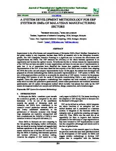
The tests performed in the data fitting functionality are based on the data inserted on the Data Fitting Worksheet Line table. The methodology consists in the creation of data using the NaviMath methods that generate random number variates for different distributions. The columns of the worksheet were populated with data associated with different distributions. Afterwards, a frequency table was constructed for each of them. In this way the random number generators and the frequency table functionality could be tested. The results of the tests can be depicted in the following graphs constructed from data generated for different distributions.
133
Uniform(2,6) 140 120
Frequency
100 80 Uniform(2,6) 60 40 20 0 1
2
3
4
5
6
7
8
9
10
Interval
Figure 35 Uniform Distribution Frequency table result Weibull(2,5) 180 160 140
frequency
120
Weibull(2,5)
100 80 60 40 20 0 1
2
3
4
5
6
7
8 9 interval
10
11
12
13
14
15
Figure 36 Weibull distribution frequency table result
134
Exponential(30) 350 300
Frequency
250 200 Exponential(30) 150 100 50 0 1
2
3
4
5
6
7
8
9 10 11 12 13 14 15
Interval
Figure 37 Exponential distribution frequency table result
Normal(0,1) 200 180 160 Frequency
140 120 100
Normal(0,1)
80 60 40 20 0 1
2
3
4
5
6
7
8
9
10 11 12 13 14 15
Interval
Figure 38 Normal distribution frequency table result
135
Triangular(1,5,3) 160 140
Frequency
120 100 80
Triangular(1,5,3)
60 40 20 0 1
2
3
4
5
6
7
8
9
10 11 12 13 14 15
Interva
Figure 39 Triangular distribution frequency table
After confirming that the distributions and the frequency table were correctly developed, the interval estimators were tested. The testing consisted in creating a testing table that had interval data, its table fields are the ones that are sought after when performing interval calculations and are shown below: Field No. 1 3 4 5 6
Field Name
Data Type
Key Start Date Start Time End Date End Time
BigInteger Date Time Date Time
Table 39 Interval Testing table fields
The data for this table was generated from the worksheet line that contained the exponential distribution data points. Each point is a time interval, then, given a starting date and time (the start of an interval), the end date and time of this interval is simply generated by adding the values from the worksheet line to the starting date and time ones. Afterwards, the next record of the testing table has its start
136
interval values equal to the end ones of the previous record. When the test table was finally populated with some test data, the function for creating the Temp Data Calculation table was executed. The results inserted on the Temp Data Calculation table should be the same as the ones from the column of the worksheet line that contain the exponential points. The script used for creating the Testing Table is shown in appendix A.
6.1.1. Goodness-of-fit tests The testing for the goodness of fit tests was simply performed by applying the test to a column of the Data Fitting Worksheet Line table that had exponentially distributed data; The result from this test are shown in the figures below, the data used for the test can be found in appendix 2.
137
Figure 40, 40 Results of the data fitting performed in exponentially distributed data
6.2.
Simulation Execution
The simulation execution testing was performed by looking at the log values from different models. The following models were created: -
Simple 1: one creator shape connected to a process and later connected to a terminator Simple 2: one creator shape connected to two sequential processes that are linked to a terminator. Router test: one creator shape connected to a router that is connected to two processes. Joiner test: two creator shapes connected to a router that is connected to a process.
All the estimators used in these tests were deterministic in order to alleviate the review process done on the simulation log. The creation shapes created one entity at a time and the process shape delayed them for two units of time. The results from parts of the logs can be found on appendix C to F.
138
For the router shape a small test script was conducted in order to test the router shape behavior. This test consisted in creating some sample data for a model in order to test the probabilistic and queue behavior of the shape. The scripts code can be found on appendix G.
139
7. Conclusions In the introduction section of this project there were some questions outlined that were used as the source of inspiration to pursue this investigation. After the completion of the design and the development of the majority of the core functionality of the prototype, it is my belief that these questions have been answered and are given as the conclusions of this project. Is simulation used in some ERP systems today and if so, in what areas? Simulation is used to a certain degree in the majority of the top players in the ERP market. Nonetheless, only few vendors implement the functionalities presented in this project and all of them implement the simulation for specific (key?) areas like manufacturing and distribution. Also, all of these vendors target the corporate segment of the market. More importantly, the inclusion of discrete event simulation applications in ERP software for small and medium size companies has not been fully developed yet. Is it possible to create a simulation module in the ERP system that I have been working on? The development of a simulation application has been proved to be possible. All the components of a standard simulation application have been developed to some degree. It is important to mention that the simplicity of the application language and the built capabilities of C/Side took care of many complications that could arise when developing a simulator in a less restricted environment. However, if performance issues are found when executing large models, the developer would have a limited set of possibilities to overcome them. An important suggestion for the application is to include the functionality present in the external components developed. This would make possible the usage of all the available business logic and functionality of the application allowing the creation of very complex models.
140
What would this system need? What functionality could it have and how could it use the potential that is already part of the ERP software? By researching some of the simulation literature the needed components were gathered and later developed. The potential of the application was not fully used since the Navision application does not allow the interaction with external components inside the development environment. Nevertheless, the fact that the simulation application was a part of the ERP system allowed a continuous flow between the data analysis and the modeling and execution phases. What do I think can be done to enhance the simulation application developed? While developing the project new ideas for functionality or enhancement were thought of. Some of them were implemented while others were just outlined. The main point behind this creative process is that the fusion of simulation with a business application gives a lot of room for inspiration since simulation is a broad concept that can be applied in many areas which can affect the application as a whole. The following list summarizes some features that could be use to enhance the current prototype:
Data Analysis -
Inclusion of more statistical distributions, especially discrete ones or user defined. A better usability for the statistical test results. For instance, a normal user would not be very familiar with terms like: chi-square test, Kolmogorovsmirnov, confidence intervals, statistical distributions and its parameters. The way to present these concepts to a “normal” user can be by using simpler terminology and wizards. For example; � Confidence intervals could be presented to the user in a wizard with a question like: How sure do you want to be on the similarities of the data and the test distributions? � When inserting parameters for the triangular distribution, instead of asking for the values for a, b and c the system could ask in a wizard: What is the most probable, minimum or maximum values for this estimator?
141
�
-
Not show any test results just give the user information about how sure he could be that the data fits a certain distribution. Include graphic capabilities to show the user how close the data is with the proposed distribution. If users are more knowledgeable in statistics, include the possibility of creating different kinds of statistical graphs. E.g. box plots, probability plots and histograms.
Estimators -
-
-
The current process of linking an estimator with the data available in the system presumes that the user has the knowledge of the table relationships and structure. This assumption is not valid for the standard user since the main interaction points he has with the application are the visible forms, menus and reports. A way to target this inconvenience would be to have a functionality linked to form fields that would allow the user to create estimators based on selections of fields performed on the form. Currently the user can use the filter capabilities for tables on the estimator card for setting some sort of attributes on the selected estimator. However, it would give more power to the user if he could insert any desired attributes to the estimators. A practical example would be that the router shape could “route” based on the created attributes. Make possible to export the data created in the temp data calculation table. In this way the data fitting can be use in an external program or send to another company for investigation. Create a communication interface in order for the external partner to send information that could be easily imported in order to link it to an estimator or create an estimator from.
Modeling -
The modeling tool could be better created as html. In this way it can be possible to create a webpage and use the modeling tool over the internet. Animation of the simulation process could help tracking the execution of the simulation. When a user creates a model and links the shapes to estimators, basically what he is doing is associating data from a table with logical processes and linking them together. This information could be use by the ERP system to establish links of functionality together, making the modeling process a tool
142
-
7.3.
that the ERP system can use to adapt to the users behavior. Furthermore, the current relations of tables or any recorded step performed by a user could be use a source for creating models. There are several process statuses that could be implemented. Some of them are: failed, on setup, starved. An idea would be to create some sort of logic units that would allow the user to give shapes certain behavior linked to user-defined statuses.
Future Work
The simulation concept and simulation software has been around for many years, most probably, at the same time ERP applications started to be developed. The fact that discrete event simulation packages are not part of the offerings of many of today’s ERP vendors, or the ones that do offer them are targeted to the high end of the ERP market, gives a strong indication that simulation is not a widely used tool nowadays. In my opinion, the main reason for the slow movement of simulation applications into the ERP arena is given by the fact that the simulation process requires a great deal of knowledge in technical areas that is not present in the majority of the consumers that constitutes the ERP market as a whole. For this reason, I believe that simulation would gain a large number of advocates if considerable efforts were made in automating the technical operations performed in a simulation study, specifically, in the data analysis process. If this process is fully automated giving reasonable results, the simulation process would basically be a modeling exercise. This could certainly help the adoption of the concept since, for instance, users that previously rejected it because of its technical barriers would now embrace it since modeling techniques are relatively ease to learn and widely used. As an example we could consider the adoption and offerings on human workflow capabilities were the user basically models the hierarchy of their organizations. For the above mentioned reasons I believe that the main area of study to focus for some future work would be in the automation of the data analysis process.
143
To conclude, I have investigated the possibilities for the inclusion of a simulation application in an ERP application. The emphasis has been made on the interaction between the data fitting and the modeling phases of simulation with ease of use as a key design criterion. In my opinion, the project has been quite successful, as the original hypotheses seem to be confirmed. Also within the limited time available it has been possible to develop a quite convincing simulation prototype.
144
Appendix A Script for creating Interval Data Function InsertTestTable() TestEstimator.DELETEALL; DataFitWrkstLine.RESET; LineNo := 1; StartDate := 010105D; StartTime := 000000T; IF DataFitWrkstLine.FIND('-') THEN BEGIN REPEAT TestEstimator.Key := LineNo; TestEstimator."Start Date" := StartDate; TestEstimator."Start Time" := StartTime; Days := DataFitWrkstLine."Column 3" * 3.6; DTVar := DTMgt.Datetime(StartDate,StartTime); DTVar := DTVar + Days; TestEstimator."End Date" := DTMgt.Datetime2Date(DTVar); TestEstimator."End Time" := DTMgt.Datetime2Time(DTVar); StartDate := TestEstimator."End Date"; StartTime := TestEstimator."End Time"; TestEstimator.INSERT; LineNo += 1; UNTIL DataFitWrkstLine.NEXT = 0; END;
145
Appendix B Exponential data used for testing the goodness-of-fit tests Line No.
Column 2
Line No.
Column 2
Line No.
Column 2
2
23
36
53
70
11
3
7
37
29
71
55
4
62
38
38
72
83
5
3
39
58
73
6
6
13
40
21
74
32
7
5
41
19
75
10
8
7
42
15
76
21
9
4
43
21
77
2
10
21
44
32
78
0
11
6
45
49
79
32
12
2
46
9
80
1
13
20
47
20
81
29
14
2
48
29
82
13
15
14
49
0
83
4
16
28
50
1
84
1
17
5
51
37
85
27
18
29
52
0
86
16
19
56
53
6
87
56
20
14
54
1
88
7
21
1
55
13
22
2
56
54
23
31
57
16
24
3
58
76
25
15
59
51
26
19
60
3
27
18
61
19
28
3
62
49
29
1
63
5
30
11
64
55
31
9
65
1
32
73
66
21
33 34
10 10
67 68
23 14
35
3
69
6
146
Appendix C Simple 1 model log Line No.
Simulation Clock
Description
1
0
2
0
Start of simulation... entity 0 has been set for Termination at shape id 0 at time 100
3
0
entity 1 has been set for Arrival at shape id 1 at time 1
4
1
entity 1 has been set for Departure at shape id 2 at time 4
5
1
Shape ID 2 has been set to busy
6
1
entity 2 has been set for Arrival at shape id 1 at time 2
7
2
entity 2 has been set on queue for shape 2
8
2
entity 3 has been set for Arrival at shape id 1 at time 3
9
3
entity 3 has been set on queue for shape 2
10
3
entity 4 has been set for Arrival at shape id 1 at time 4
11
4
entity 2 has been taken from the queue on shape ID 2
12
4
entity 2 has been set for Departure at shape id 2 at time 7
13
4
entity 1 has terminated the run
14
4
entity 4 has been set on queue for shape 2
15
4
entity 5 has been set for Arrival at shape id 1 at time 5
16
5
entity 5 has been set on queue for shape 2
17
5
entity 6 has been set for Arrival at shape id 1 at time 6
18
6
entity 6 has been set on queue for shape 2
19
6
entity 7 has been set for Arrival at shape id 1 at time 7
20
7
entity 3 has been taken from the queue on shape ID 2
21
7
entity 3 has been set for Departure at shape id 2 at time 10
22
7
entity 2 has terminated the run
Date 27-102005 27-102005 27-102005 27-102005 27-102005 27-102005 27-102005 27-102005 27-102005 27-102005 27-102005 27-102005 27-102005 27-102005 27-102005 27-102005 27-102005 27-102005 27-102005 27-102005 27-102005 27-10-
Time 21:05:06 21:05:06 21:05:06 21:05:06 21:05:06 21:05:06 21:05:06 21:05:06 21:05:06 21:05:06 21:05:06 21:05:06 21:05:06 21:05:06 21:05:06 21:05:06 21:05:06 21:05:06 21:05:06 21:05:06 21:05:06 21:05:06
147
2005 23
7
entity 7 has been set on queue for shape 2
24
7
entity 8 has been set for Arrival at shape id 1 at time 8
25
8
entity 8 has been set on queue for shape 2
26
8
entity 9 has been set for Arrival at shape id 1 at time 9
27
9
entity 9 has been set on queue for shape 2
28
9
entity 10 has been set for Arrival at shape id 1 at time 10
29
10
entity 4 has been taken from the queue on shape ID 2
30
10
entity 4 has been set for Departure at shape id 2 at time 13
31
10
entity 3 has terminated the run
32
10
entity 10 has been set on queue for shape 2
33
10
entity 11 has been set for Arrival at shape id 1 at time 11
34
11
entity 11 has been set on queue for shape 2
35
11
entity 12 has been set for Arrival at shape id 1 at time 12
36
12
entity 12 has been set on queue for shape 2
37
12
entity 13 has been set for Arrival at shape id 1 at time 13
38
13
entity 5 has been taken from the queue on shape ID 2
39
13
entity 5 has been set for Departure at shape id 2 at time 16
40
13
entity 4 has terminated the run
41
13
entity 13 has been set on queue for shape 2
42
13
entity 14 has been set for Arrival at shape id 1 at time 14
43
14
entity 14 has been set on queue for shape 2
27-102005 27-102005 27-102005 27-102005 27-102005 27-102005 27-102005 27-102005 27-102005 27-102005 27-102005 27-102005 27-102005 27-102005 27-102005 27-102005 27-102005 27-102005 27-102005 27-102005 27-102005
21:05:06 21:05:06 21:05:06 21:05:06 21:05:06 21:05:06 21:05:06 21:05:06 21:05:06 21:05:06 21:05:06 21:05:06 21:05:06 21:05:06 21:05:06 21:05:06 21:05:06 21:05:06 21:05:06 21:05:06 21:05:06
148
Appendix D Simple 2 model log Line No.
Simulation Clock
Description
1
0
2
0
Start of simulation... entity 0 has been set for Termination at shape id 0 at time 100
3
0
entity 1 has been set for Arrival at shape id 1 at time 1
4
1
entity 1 has been set for Departure at shape id 2 at time 5
5
1
Shape ID 2 has been set to busy
6
1
entity 2 has been set for Arrival at shape id 1 at time 2
7
2
entity 2 has been set on queue for shape 2
8
2
entity 3 has been set for Arrival at shape id 1 at time 3
9
3
entity 3 has been set on queue for shape 2
10
3
entity 4 has been set for Arrival at shape id 1 at time 4
11
4
entity 4 has been set on queue for shape 2
12
4
entity 5 has been set for Arrival at shape id 1 at time 5
13
5
entity 1 has been set for Departure at shape id 3 at time 7
14
5
Shape ID 3 has been set to busy
15
5
entity 2 has been taken from the queue on shape ID 2
16
5
entity 2 has been set for Departure at shape id 2 at time 9
17
5
entity 5 has been set on queue for shape 2
18
5
entity 6 has been set for Arrival at shape id 1 at time 6
19
6
entity 6 has been set on queue for shape 2
20
6
entity 7 has been set for Arrival at shape id 1 at time 7
21
7
Shape ID 3 has been set to idle again
22
7
entity 1 has terminated the run
23
7
entity 7 has been set on queue for shape 2
Date 29-102005 29-102005 29-102005 29-102005 29-102005 29-102005 29-102005 29-102005 29-102005 29-102005 29-102005 29-102005 29-102005 29-102005 29-102005 29-102005 29-102005 29-102005 29-102005 29-102005 29-102005 29-102005 29-102005
Time 17:45:51 17:45:51 17:45:51 17:45:51 17:45:51 17:45:51 17:45:51 17:45:51 17:45:51 17:45:51 17:45:51 17:45:51 17:45:51 17:45:51 17:45:51 17:45:51 17:45:51 17:45:51 17:45:51 17:45:51 17:45:51 17:45:51 17:45:51
149
24
7
entity 8 has been set for Arrival at shape id 1 at time 8
25
8
entity 8 has been set on queue for shape 2
26
8
entity 9 has been set for Arrival at shape id 1 at time 9
27
9
entity 2 has been set for Departure at shape id 3 at time 11
28
9
Shape ID 3 has been set to busy
29
9
entity 3 has been taken from the queue on shape ID 2
30
9
entity 3 has been set for Departure at shape id 2 at time 13
31
9
entity 9 has been set on queue for shape 2
32
9
entity 10 has been set for Arrival at shape id 1 at time 10
33
10
entity 10 has been set on queue for shape 2
34
10
entity 11 has been set for Arrival at shape id 1 at time 11
35
11
Shape ID 3 has been set to idle again
36
11
entity 2 has terminated the run
37
11
entity 11 has been set on queue for shape 2
38
11
entity 12 has been set for Arrival at shape id 1 at time 12
39
12
entity 12 has been set on queue for shape 2
40
12
entity 13 has been set for Arrival at shape id 1 at time 13
41
13
entity 3 has been set for Departure at shape id 3 at time 15
42
13
Shape ID 3 has been set to busy
43
13
entity 4 has been taken from the queue on shape ID 2
44
13
entity 4 has been set for Departure at shape id 2 at time 17
45
13
entity 13 has been set on queue for shape 2
46
13
entity 14 has been set for Arrival at shape id 1 at time 14
47
14
entity 14 has been set on queue for shape 2
48
14
entity 15 has been set for Arrival at shape id 1 at time 15
29-102005 29-102005 29-102005 29-102005 29-102005 29-102005 29-102005 29-102005 29-102005 29-102005 29-102005 29-102005 29-102005 29-102005 29-102005 29-102005 29-102005 29-102005 29-102005 29-102005 29-102005 29-102005 29-102005 29-102005 29-102005
49
15
Shape ID 3 has been set to idle again
29-10-
17:45:51 17:45:51 17:45:51 17:45:51 17:45:51 17:45:51 17:45:51 17:45:51 17:45:51 17:45:51 17:45:51 17:45:51 17:45:51 17:45:51 17:45:51 17:45:51 17:45:51 17:45:51 17:45:51 17:45:51 17:45:51 17:45:51 17:45:51 17:45:51 17:45:51 17:45:51
150
2005 50
15
entity 3 has terminated the run
51
15
entity 15 has been set on queue for shape 2
52
15
entity 16 has been set for Arrival at shape id 1 at time 16
53
16
entity 16 has been set on queue for shape 2
54
16
entity 17 has been set for Arrival at shape id 1 at time 17
55
17
entity 4 has been set for Departure at shape id 3 at time 19
56
17
Shape ID 3 has been set to busy
57
17
entity 5 has been taken from the queue on shape ID 2
58
17
entity 5 has been set for Departure at shape id 2 at time 21
59
17
entity 17 has been set on queue for shape 2
60
17
entity 18 has been set for Arrival at shape id 1 at time 18
61
18
entity 18 has been set on queue for shape 2
62
18
entity 19 has been set for Arrival at shape id 1 at time 19
63
19
Shape ID 3 has been set to idle again
64
19
entity 4 has terminated the run
65
19
entity 19 has been set on queue for shape 2
66
19
entity 20 has been set for Arrival at shape id 1 at time 20
67
20
entity 20 has been set on queue for shape 2
68
20
entity 21 has been set for Arrival at shape id 1 at time 21
69
21
entity 5 has been set for Departure at shape id 3 at time 23
29-102005 29-102005 29-102005 29-102005 29-102005 29-102005 29-102005 29-102005 29-102005 29-102005 29-102005 29-102005 29-102005 29-102005 29-102005 29-102005 29-102005 29-102005 29-102005 29-102005
17:45:51 17:45:51 17:45:51 17:45:51 17:45:51 17:45:51 17:45:51 17:45:51 17:45:51 17:45:51 17:45:51 17:45:51 17:45:51 17:45:51 17:45:51 17:45:51 17:45:51 17:45:51 17:45:51 17:45:51
151
Appendix E Joiner Test model log Line No.
Simulation Clock
Description
1
0
Start of simulation...
2
0
entity 0 has been set for Termination at shape id 0 at time 100
3
0
entity 1 has been set for Arrival at shape id 1 at time 1
4
0
entity 2 has been set for Arrival at shape id 2 at time 1
5
1
6
1
entity 3 has been set for Arrival at shape id 1 at time 2 Entity ID 4 has been created on Joiner no 3, The joiner has been flushed
7
1
entity 4 has been set for Departure at shape id 4 at time 5
8
1
Shape ID 4 has been set to busy
9
1
entity 5 has been set for Arrival at shape id 2 at time 2
10
2
entity 3 has been set on queue for shape 3
11
2
12
2
entity 6 has been set for Arrival at shape id 1 at time 3 Entity ID 7 has been created on Joiner no 3, The joiner has been flushed
13
2
entity 7 has been set on queue for shape 4
14
2
entity 8 has been set for Arrival at shape id 2 at time 3
15
3
entity 6 has been set on queue for shape 3
16
3
17
3
entity 9 has been set for Arrival at shape id 1 at time 4 Entity ID 10 has been created on Joiner no 3, The joiner has been flushed
18
3
entity 10 has been set on queue for shape 4
19
3
entity 11 has been set for Arrival at shape id 2 at time 4
20
4
entity 9 has been set on queue for shape 3
21
4
22
4
entity 12 has been set for Arrival at shape id 1 at time 5 Entity ID 13 has been created on Joiner no 3, The joiner has been flushed
Date 29-102005 29-102005 29-102005 29-102005 29-102005 29-102005 29-102005 29-102005 29-102005 29-102005 29-102005 29-102005 29-102005 29-102005 29-102005 29-102005 29-102005 29-102005 29-102005 29-102005 29-102005 29-102005
Time 4:44:42 4:44:42 4:44:42 4:44:42 4:44:42 4:44:42 4:44:42 4:44:42 4:44:42 4:44:42 4:44:42 4:44:42 4:44:42 4:44:42 4:44:42 4:44:42 4:44:42 4:44:42 4:44:42 4:44:42 4:44:42 4:44:42
152
23
4
entity 13 has been set on queue for shape 4
24
4
entity 14 has been set for Arrival at shape id 2 at time 5
25
5
entity 7 has been taken from the queue on shape ID 4
26
5
entity 7 has been set for Departure at shape id 4 at time 9
27
5
entity 4 has terminated the run
28
5
entity 12 has been set on queue for shape 3
29
5
30
5
entity 15 has been set for Arrival at shape id 1 at time 6 Entity ID 16 has been created on Joiner no 3, The joiner has been flushed
31
5
entity 16 has been set on queue for shape 4
32
5
entity 17 has been set for Arrival at shape id 2 at time 6
33
6
entity 15 has been set on queue for shape 3
34
6
35
6
entity 18 has been set for Arrival at shape id 1 at time 7 Entity ID 19 has been created on Joiner no 3, The joiner has been flushed
36
6
entity 19 has been set on queue for shape 4
37
6
entity 20 has been set for Arrival at shape id 2 at time 7
38
7
entity 18 has been set on queue for shape 3
39
7
40
7
entity 21 has been set for Arrival at shape id 1 at time 8 Entity ID 22 has been created on Joiner no 3, The joiner has been flushed
41
7
entity 22 has been set on queue for shape 4
42
7
entity 23 has been set for Arrival at shape id 2 at time 8
43
8
entity 21 has been set on queue for shape 3
44
8
45
8
entity 24 has been set for Arrival at shape id 1 at time 9 Entity ID 25 has been created on Joiner no 3, The joiner has been flushed
46
8
entity 25 has been set on queue for shape 4
47
8
entity 26 has been set for Arrival at shape id 2 at time 9
29-102005 29-102005 29-102005 29-102005 29-102005 29-102005 29-102005 29-102005 29-102005 29-102005 29-102005 29-102005 29-102005 29-102005 29-102005 29-102005 29-102005 29-102005 29-102005 29-102005 29-102005 29-102005 29-102005 29-102005 29-102005
48
9
entity 10 has been taken from the queue on shape ID 4
29-10-
4:44:42 4:44:42 4:44:42 4:44:42 4:44:42 4:44:42 4:44:42 4:44:42 4:44:42 4:44:42 4:44:42 4:44:42 4:44:42 4:44:42 4:44:42 4:44:42 4:44:42 4:44:42 4:44:42 4:44:42 4:44:42 4:44:42 4:44:42 4:44:42 4:44:42
153
2005 49
9
entity 10 has been set for Departure at shape id 4 at time 13
50
9
entity 7 has terminated the run
51
9
entity 24 has been set on queue for shape 3
52
9
53
9
entity 27 has been set for Arrival at shape id 1 at time 10 Entity ID 28 has been created on Joiner no 3, The joiner has been flushed
54
9
entity 28 has been set on queue for shape 4
55
9
entity 29 has been set for Arrival at shape id 2 at time 10
56
10
entity 27 has been set on queue for shape 3
57
10
58
10
entity 30 has been set for Arrival at shape id 1 at time 11 Entity ID 31 has been created on Joiner no 3, The joiner has been flushed
59
10
entity 31 has been set on queue for shape 4
60
10
entity 32 has been set for Arrival at shape id 2 at time 11
61
11
entity 30 has been set on queue for shape 3
62
11
63
11
entity 33 has been set for Arrival at shape id 1 at time 12 Entity ID 34 has been created on Joiner no 3, The joiner has been flushed
64
11
entity 34 has been set on queue for shape 4
65
11
entity 35 has been set for Arrival at shape id 2 at time 12
66
12
entity 33 has been set on queue for shape 3
67
12
68
12
entity 36 has been set for Arrival at shape id 1 at time 13 Entity ID 37 has been created on Joiner no 3, The joiner has been flushed
69
12
entity 37 has been set on queue for shape 4
70
12
entity 38 has been set for Arrival at shape id 2 at time 13
71
13
entity 13 has been taken from the queue on shape ID 4
72
13
entity 13 has been set for Departure at shape id 4 at time 17
73
13
entity 10 has terminated the run
29-102005 29-102005 29-102005 29-102005 29-102005 29-102005 29-102005 29-102005 29-102005 29-102005 29-102005 29-102005 29-102005 29-102005 29-102005 29-102005 29-102005 29-102005 29-102005 29-102005 29-102005 29-102005 29-102005 29-102005 29-102005
4:44:42 4:44:42 4:44:42 4:44:42 4:44:42 4:44:42 4:44:42 4:44:42 4:44:42 4:44:42 4:44:42 4:44:42 4:44:42 4:44:42 4:44:42 4:44:42 4:44:42 4:44:42 4:44:42 4:44:42 4:44:42 4:44:42 4:44:42 4:44:42 4:44:42 4:44:42
154
74
13
entity 36 has been set on queue for shape 3
75
13
76
13
entity 39 has been set for Arrival at shape id 1 at time 14 Entity ID 40 has been created on Joiner no 3, The joiner has been flushed
77
13
entity 40 has been set on queue for shape 4
78
13
entity 41 has been set for Arrival at shape id 2 at time 14
79
14
entity 39 has been set on queue for shape 3
80
14
entity 42 has been set for Arrival at shape id 1 at time 15
29-102005 29-102005 29-102005 29-102005 29-102005 29-102005 29-102005
4:44:42 4:44:42 4:44:42 4:44:42 4:44:42 4:44:42 4:44:42
155
Appendix F Router Test model log Line No.
Simulation Clock
Description
1
0
2
0
Start of simulation... entity 0 has been set for Termination at shape id 0 at time 120
3
0
entity 1 has been set for Arrival at shape id 1 at time 3
4
3
The router 2 chose to route to shape no: 3
5
3
entity 1 has been set for Departure at shape id 3 at time 7
6
3
Shape ID 3 has been set to busy
7
3
entity 2 has been set for Arrival at shape id 1 at time 6
8
6
The router 2 chose to route to shape no: 3
9
6
entity 2 has been set on queue for shape 3
10
6
entity 3 has been set for Arrival at shape id 1 at time 9
11
7
entity 2 has been taken from the queue on shape ID 3
12
7
entity 2 has been set for Departure at shape id 3 at time 11
13
7
entity 1 has terminated the run
14
9
The router 2 chose to route to shape no: 4
15
9
entity 3 has been set for Departure at shape id 4 at time 11
16
9
Shape ID 4 has been set to busy
17
9
entity 4 has been set for Arrival at shape id 1 at time 12
18
11
Shape ID 3 has been set to idle again
19
11
entity 2 has terminated the run
20
11
Shape ID 4 has been set to idle again
21
11
entity 3 has terminated the run
22
12
The router 2 chose to route to shape no: 4
Date 29-102005 29-102005 29-102005 29-102005 29-102005 29-102005 29-102005 29-102005 29-102005 29-102005 29-102005 29-102005 29-102005 29-102005 29-102005 29-102005 29-102005 29-102005 29-102005 29-102005 29-102005 29-102005
Time 4:46:02 4:46:02 4:46:02 4:46:02 4:46:02 4:46:02 4:46:02 4:46:02 4:46:02 4:46:02 4:46:02 4:46:02 4:46:02 4:46:02 4:46:02 4:46:02 4:46:02 4:46:02 4:46:02 4:46:02 4:46:02 4:46:02
156
23
12
entity 4 has been set for Departure at shape id 4 at time 14
24
12
Shape ID 4 has been set to busy
25
12
entity 5 has been set for Arrival at shape id 1 at time 15
26
14
Shape ID 4 has been set to idle again
27
14
entity 4 has terminated the run
28
15
The router 2 chose to route to shape no: 4
29
15
entity 5 has been set for Departure at shape id 4 at time 17
30
15
Shape ID 4 has been set to busy
31
15
entity 6 has been set for Arrival at shape id 1 at time 18
32
17
Shape ID 4 has been set to idle again
33
17
entity 5 has terminated the run
34
18
The router 2 chose to route to shape no: 3
35
18
entity 6 has been set for Departure at shape id 3 at time 22
36
18
Shape ID 3 has been set to busy
37
18
entity 7 has been set for Arrival at shape id 1 at time 21
38
21
The router 2 chose to route to shape no: 3
39
21
entity 7 has been set on queue for shape 3
40
21
entity 8 has been set for Arrival at shape id 1 at time 24
41
22
entity 7 has been taken from the queue on shape ID 3
42
22
entity 7 has been set for Departure at shape id 3 at time 26
43
22
entity 6 has terminated the run
44
24
The router 2 chose to route to shape no: 3
45
24
entity 8 has been set on queue for shape 3
46
24
entity 9 has been set for Arrival at shape id 1 at time 27
47
26
entity 8 has been taken from the queue on shape ID 3
29-102005 29-102005 29-102005 29-102005 29-102005 29-102005 29-102005 29-102005 29-102005 29-102005 29-102005 29-102005 29-102005 29-102005 29-102005 29-102005 29-102005 29-102005 29-102005 29-102005 29-102005 29-102005 29-102005 29-102005 29-102005
48
26
entity 8 has been set for Departure at shape id 3 at time 30
29-10-
4:46:02 4:46:02 4:46:02 4:46:02 4:46:02 4:46:02 4:46:02 4:46:02 4:46:02 4:46:02 4:46:02 4:46:02 4:46:02 4:46:02 4:46:02 4:46:02 4:46:02 4:46:02 4:46:03 4:46:03 4:46:03 4:46:03 4:46:03 4:46:03 4:46:03 4:46:03
157
2005 49
26
entity 7 has terminated the run
50
27
The router 2 chose to route to shape no: 3
51
27
entity 9 has been set on queue for shape 3
52
27
entity 10 has been set for Arrival at shape id 1 at time 30
53
30
entity 9 has been taken from the queue on shape ID 3
54
30
entity 9 has been set for Departure at shape id 3 at time 34
55
30
entity 8 has terminated the run
56
30
The router 2 chose to route to shape no: 4
57
30
entity 10 has been set for Departure at shape id 4 at time 32
58
30
Shape ID 4 has been set to busy
59
30
entity 11 has been set for Arrival at shape id 1 at time 33
60
32
Shape ID 4 has been set to idle again
61
32
entity 10 has terminated the run
62
33
The router 2 chose to route to shape no: 4
63
33
entity 11 has been set for Departure at shape id 4 at time 35
64
33
Shape ID 4 has been set to busy
65
33
entity 12 has been set for Arrival at shape id 1 at time 36
66
34
Shape ID 3 has been set to idle again
67
34
entity 9 has terminated the run
68
35
Shape ID 4 has been set to idle again
69
35
entity 11 has terminated the run
70
36
The router 2 chose to route to shape no: 3
71
36
entity 12 has been set for Departure at shape id 3 at time 40
72
36
Shape ID 3 has been set to busy
73
36
entity 13 has been set for Arrival at shape id 1 at time 39
29-102005 29-102005 29-102005 29-102005 29-102005 29-102005 29-102005 29-102005 29-102005 29-102005 29-102005 29-102005 29-102005 29-102005 29-102005 29-102005 29-102005 29-102005 29-102005 29-102005 29-102005 29-102005 29-102005 29-102005 29-102005
4:46:03 4:46:03 4:46:03 4:46:03 4:46:03 4:46:03 4:46:03 4:46:03 4:46:03 4:46:03 4:46:03 4:46:03 4:46:03 4:46:03 4:46:03 4:46:03 4:46:03 4:46:03 4:46:03 4:46:03 4:46:03 4:46:03 4:46:03 4:46:03 4:46:03
158
74
39
The router 2 chose to route to shape no: 3
75
39
entity 13 has been set on queue for shape 3
76
39
entity 14 has been set for Arrival at shape id 1 at time 42
77
40
entity 13 has been taken from the queue on shape ID 3
78
40
entity 13 has been set for Departure at shape id 3 at time 44
79
40
entity 12 has terminated the run
80
42
The router 2 chose to route to shape no: 3
29-102005 29-102005 29-102005 29-102005 29-102005 29-102005 29-102005
4:46:03 4:46:03 4:46:03 4:46:03 4:46:03 4:46:03 4:46:03
159
Appendix G Test Script for the Router Shape Function TestNonEmptyQueueRouter() SimModelDetail."Model Code" := 'TestRouter12345'; SimModelDetail."Shape ID" := 1 ; SimModelDetail."Probabilistic Router" := FALSE; SimModelDetail.INSERT; FOR ShapeID := 2 TO 4 DO BEGIN ModelRouterValue."Model Code" := 'TestRouter12345'; ModelRouterValue."Shape ID" := 1; ModelRouterValue."Connect to Shape ID" := ShapeID; ModelRouterValue.INSERT; END; ShapeQueue.DELETEALL; EntityID := 0; FOR ShapeID := 2 TO 4 DO BEGIN EntityID += 1; CASE ShapeID OF 2:FOR x := 1 TO 20 DO BEGIN InsertEntityOnQueue(ShapeID,EntityID); END; 3:FOR x := 1 TO 10 DO BEGIN InsertEntityOnQueue(ShapeID,EntityID); END; 4:FOR x := 1 TO 5 DO BEGIN InsertEntityOnQueue(ShapeID,EntityID); END; END; END; SimEngine.SetModelCode('TestRouter12345'); MESSAGE('Next Shape '+FORMAT(SimEngine.GetNextShapeFromRouter(1))); Function TestEmptyQueueRouter() SimModelDetail.SETRANGE("Model Code",'TestRouter12345'); SimModelDetail.DELETEALL; SimModelDetail."Model Code" := 'TestRouter12345'; SimModelDetail."Shape ID" := 1 ; SimModelDetail."Probabilistic Router" := FALSE; SimModelDetail.INSERT;
selected:
160
FOR ShapeID := 2 TO 4 DO BEGIN ModelRouterValue."Model Code" := 'TestRouter12345'; ModelRouterValue."Shape ID" := 1; ModelRouterValue."Connect to Shape ID" := ShapeID; ModelRouterValue.INSERT; END; SimEngine.SetModelCode('TestRouter12345'); FOR x := 1 TO 1 DO BEGIN MESSAGE('Next Shape '+FORMAT(SimEngine.GetNextShapeFromRouter(1))); END;
selected:
Function TestProbRouter() SimModelDetail.SETRANGE("Model Code",'TestRouter12345'); SimModelDetail.DELETEALL; SimModelDetail."Model Code" := 'TestRouter12345'; SimModelDetail."Shape ID" := 1 ; SimModelDetail."Probabilistic Router" := TRUE; SimModelDetail.INSERT; FOR ShapeID := 2 TO 4 DO BEGIN ModelRouterValue."Model Code" := 'TestRouter12345'; ModelRouterValue."Shape ID" := 1; CASE ShapeID OF 2:ModelRouterValue.Probability := 0.125; 3:ModelRouterValue.Probability := 0.325; 4:ModelRouterValue.Probability := 0.550; END; ModelRouterValue."Connect to Shape ID" := ShapeID; ModelRouterValue.INSERT; END; SimEngine.SetModelCode('TestRouter12345'); FOR x := 1 TO 5 DO BEGIN Rnd := RANDOM(1001); MESSAGE(FORMAT((Rnd-1)/1000)); SimEngine.SetRandomNo(Rnd); MESSAGE('Next Shape '+FORMAT(SimEngine.GetNextShapeFromRouter(1))); END; InsertEntityOnQueue(ShapeID : Integer;EntityID : Integer) ShapeQueue.RESET; ShapeQueue.SETRANGE("Shape ID",ShapeID); IF ShapeQueue.FIND('+') THEN LineNo := ShapeQueue."Line No." + 1 ELSE LineNo := 1;
selected:
161
ShapeQueue.INIT; ShapeQueue."Shape ID" := ShapeID; ShapeQueue."Line No." := LineNo; ShapeQueue."Entity ID" := EntityID; ShapeQueue.INSERT;
162
References [1] Law, A.M and Kelton, W. David, Simulation Modeling and Analysis Second Edition, 1991, McGraw Hill Inc. [2] Banks, Jerry and Carson John S., Discrete-Event Simulation, Prentice-Hall Inc. [3] David W Sabo, “Frequency Tables”. http://www.math.bcit.ca/faculty/david_sabo/apples/math2441/section2/freqtables/fr eqtables.htm [4] New for August 2002, Textile/Clothing Technology Corporation, 2005. Web Resource :http://www.techexchange.com/BreakingNews/arc/0802.html [5] Business Intelligence marketing material, Sap AS., 2005. Web Resouce: http://www.sap.com/solutions/netweaver/ businessintelligence/index.epx [6] Supply Chain Management, SSA global technologies, inc, 2005. Web Resource: http://www.ssaglobal.com/solutions/scm/manscheduling.aspx [7] Eric W. Weisstein. "Normal Distribution." From MathWorld--A Wolfram Web Resource. http://mathworld.wolfram.com/NormalDistribution.html [8] Eric W. Weisstein. "Central Limit Theorem." From MathWorld--A Wolfram Web Resource. http://mathworld.wolfram.com/CentralLimitTheorem.html [9] The Weibull Distribution, NIST/SEMATECH e-Handbook of Statistical Methods, http://www.itl.nist.gov/div898/handbook/eda/section3/eda3668.htm, 2005. [10] History of Navision, Accounting Software advisor, 2005 Web Resource.http://www.mbsadvisor.com/navision/history.htm
163
[11] ERP software, Wikipedia the On-line encyclopedia, 2005 Web Resource: http://en.wikipedia.org/wiki/ERP_software. [12]Microsoft Business Solutions web site, 2005. Web Resource: http://www.microsoft.com/BusinessSolutions [13] Simulation, Sage, 2005. Web Resource: http://www.sage.de/public2/smb/prodloes/office_line/ produktion_simulation.asp [14] Peoplesoft Workforce Rewards, Oracle 2005, Web Resource: http://www.oracle.com/applications/performance-management/ ent/module/wrkfrc_rewards.html [15] Oracle BPEL Process Manager, Web Resource: http://www.oracle.com/technology/products/ias/bpel/index.html