A Sparse Frisch-Newton Algorithm for Quantile Regression

A FRISCH-NEWTON ALGORITHM FOR SPARSE QUANTILE REGRESSION ROGER KOENKER AND PIN NG Abstract. Recent experience has shown that interior-point methods using a log barrier approach are far superior to classical simplex methods for computing solutions to large parametric quantile regression problems. In many large empirical applications, the design matrix has a very sparse structure. A typical example is the classical fixed-effect model for panel data where the parametric dimension of the model can be quite large, but the number of non-zero elements is quite small. Adopting recent developments in sparse linear algebra we introduce a modified version of the Frisch-Newton algorithm for quantile regression described in Portnoy and Koenker (1997). The new algorithm substantially reduces the storage (memory) requirements and increases computational speed. The modified algorithm also facilitates the development of nonparametric quantile regression methods. The pseudo design matrices employed in nonparametric quantile regression smoothing are inherently sparse in both the fidelity and roughness penalty components. Exploiting the sparse structure of these problems opens up a whole range of new possibilities for multivariate smoothing on large data sets via ANOVA-type decomposition and partial linear models.

1. Introduction After almost three decades of development quantile regression is gradually emerging as a fundamental tool of applied statistics. Complementing the use of least squares methods for estimating conditional mean models, quantile regression not only offers a more robust alternative for estimating the central tendency of the response, but also allows researchers to explore more fully the conditional distribution of the response. In the classical regression framework, the conditional mean E (Y |X = x) is estimated by the least squares method. Unless one is willing to make strong distributional assumptions on the conditional distribution of the response, least squares methods do not provide any information beyond the conditional mean. Quantile regression generalizes the idea of median regression to estimation of other conditional quantile functions by minimizing weighted sums of absolute residuals and, hence, enable investigators to examine the effect of various covariates on other quantiles of the response. Median regression, introduced by Boscovich in the mid-18th century, and championed by Laplace at the end of that century, seeks to estimate parametric statistical Key words and phrases. Quantile regression, interior-point algorithm, sparse linear algebra. Version: August 25, 2004. Corresponding author: Pin Ng, College of Business Administration, Northern Arizona University, 70 McConnell Dr, P.O. Box 15066, Flagstaff, AZ 86011-5066. This research was partially supported by NSF grant SES-02-40781. 1

2

Sparse Frisch Newton Algorithm

models by minimizing sums of absolute residuals. From its inception it has been recognized as a challenging computational problem. With the discovery of least squares methods by Gauss and Legendre at the end of the 18th century, it fell into a benign neglect, only to be revived by Edgeworth at the end of the 19th century, and again with the discovery of the simplex algorithm for linear programming in the late 1940’s. The last decade has seen a flurry of quantile regression applications in a wide variety of disciplines including economics, finance, demography, sociology and social policy, education, political science, ecology, environmental science, biostatistics and medicine. Until quite recently, simplex based methods, notably the algorithm of Barrodale and Roberts (1974), offered the only viable approach to computation for quantile regression. Koenker and D’Orey (1987, 1993) describe this approach and some related computational methods for inference. The introduction of interior point methods by Karmarker (1984) unleashed a fundamental shift in the paradigm of computation for linear programming. Significant progress has been made over the last decade to improve the computational efficiency of interior point methods for linear programming. See Gonzaga (1992), Lustig, Marsten and Shanno (1994), and Wright (1997) for surveys of the development of interior point methods. Primal-dual interior point algorithms are competitive with classical simplex methods for small to moderate size problems and far superior for large problems. Portnoy and Koenker (1997) showed that interior point methods combined with careful preprocessing could effectively reduce the computational effort of quantile regression problems to that of the corresponding least squares problems. But their approach was designed for “long, thin problems”, that is for problems with large sample size, but only a relatively small number of parameters. In many large empirical applications of quantile regressions, however, the parametric dimension of the model can be quite large. Particularly challenging are large-scale problems that involve nonparametric function estimation, see e.g., Koenker, Ng and Portnoy (1994), He, Ng and Portnoy (1998), He and Ng (1999) and Koenker and Mizera (2004). Often though, such problems have a design matrix that has a very sparse structure. A typical example is the classical fixed-effect model for panel data where the parametric dimension of the model can be quite large, due to a large number of indicator variables and their interactions, but the number of non-zero elements in the design matrix can be quite small. The design matrices arising in nonparametric quantile regression smoothing problems are also inherently sparse in both their fidelity and roughness penalty components. These problems call for new methods that rely on effective exploitation of the sparsity of the matrix structure of the problems to achieve improvements in computational efficiency. With the emergence of massive-scale data mining in business, economic and biological applications there is a compelling need for more efficient computational methods. In this paper we adapt recent developments in sparse linear algebra to introduce a modified version of the Frisch-Newton algorithm for quantile regression described

Koenker and Ng

3

in Portnoy and Koenker (1997). The new algorithm utilizes the BLAS-like routines for sparse matrices available from Saad (1994) and adapted in Koenker and Ng (2002), and the block sparse Cholesky algorithm of Ng and Peyton (1993). Our implementation substantially reduces storage (memory) requirements and increases computational speed. Exploiting the sparse structure opens up a whole range of new applications for multivariate smoothing on large data sets via ANOVA-type decomposition and partial linear models. 2. Quantiles Regression Given τ ∈ [0, 1] and n observations on the dependent variable yi and the p-variate independent variable xi , the τ -th parametric linear regression quantile b is defined as the solution to n X (1) minp ρτ (yi − x> i b) b∈R

i=1

where ρτ (u) = u(τ − I(u < 0)). As demonstrated in Koenker and Ng (2004), (1) can be rewritten as the following linear program with e denoting an n-vector of ones: (2)

min {τ e> u + (1 − τ )e> v|Xb + u − v = y,

(u> ,v> ,b> )

>

>

>

p (u , v , b ) ∈ R2n + ×R }

Here, u and v are the positive and negative parts of the regression residuals. The dual of (2) is max{y >d|X > d = (1 − τ )X > e,

(3)

d

d ∈ [0, 1]n }

where [0, 1]n denotes the n-fold Cartesian product of the unit interval, and d may be interpreted as a vector of Lagrange multipliers associated with the linear equality constraints of the primal problem in (1). It is this bounded variables dual linear program in (3) that we will solve using the interior point methods. 3. The Frisch-Newton Algorithm Lustig, Marsten and Shanno (1992, 1994) express a linear program primal-dual pair as x ∈ Rn }  > > > p {b> y|A> y + z − w = c, z , w , y ∈ R2n + × R }.

(4)

min{c> x|Ax = b, 0 ≤ x ≤ u,

(5)

max (z > ,w> ,y> )

x

Note that the dual in (3) that we want to solve corresponds to the primal in (4) so > > that −y, d, (1 − τ ) X e, and X in (3) correspond, respectively, to c, x, b, and A in (4). The log-barrier form of the Lagrangian for the primal problem in (4) is, X X L = c> x − y > (Ax − b) − w > (u − x − s) − µ( log xi + log si ),

Sparse Frisch Newton Algorithm

4

for µ > 0. The last log-barrier term in the expression above guarantees that (x, s) stays away from the boundary of the positive orthant. The strategy is to gradually relax the barrier parameter µ, letting it tend toward zero as the duality gap c> x − b> y > 0 closes and we approach the optimal solution. Writing z = µX −1 e and differentiating with respect to (y > , x> , s> , w > )> , the classical Karush-Kuhn-Tucker conditions for optimality are 

  g (ξ) =   

(6)

A> y + z − w − c Ax − b x+s−u XZe − µe SW e − µe



  =0  

where the upper case letters are diagonal matrices with the corresponding lower case vectors as their diagonal elements, so for example X = diag (x). Given an initial point, ξ = (y > , z > , x> , s> , w > )> , of the primal-dual variables, the Newton approximation to (6) is g(ξk+1) ≈ ∇ξ g(ξ)dξ + g(ξ).
> We choose a descent direction dξ = dy > , dz > , dx> , ds> , dw > by setting the above Newton approximation equal zero. The resulting linear system we obtain is  (7)

    

   A> I 0 0 −I dy A> y + z − w − c    0 0 A 0 0  Ax − b   dz      0 0 I I 0   dx  = −  x +s−u      0 X Z 0 0 ds XZe − µe 0 0 0 W S dw SW e − µe





    =    

r1 r2 r3 r4 r5

     

All primal-dual log barrier form of interior point algorithms involve generating sequences of the primal-dual variables and iterating until the duality gap becomes smaller than a specified tolerance. Frisch (1955) was a pioneering advocate of the log-barrier method for solving linear programming problems, so Portnoy and Koenker (1997) dub their primal-dual log barrier interior point implementation for quantile regression a Frisch-Newton algorithm. The Frisch-Newton algorithm we implement here consists of three components at each iteration: (i) an affine-scaling “predictor” direction is first computed, (ii) separate primal and dual step lengths are then obtained and the barrier parameter µ is updated so that, (iii) a “corrected” direction can be computed and a step taken along the corrected direction. Affine-scaling predictor direction First, the affine-scaling predictor steps are obtain by solving (7) with µ = 0. After some linear algebra that can be

Koenker and Ng

5

found in Koenker and Ng (2004), the predictor steps can be obtained as dy = (AQ−1 A> )−1 [˜ r2 + AQ−1 r˜1 ] dx = Q−1 (A> dy − r˜1 ) (8)

ds = −dx
dz = −z − X −1 Zdx = −Z e + X −1 dx
dw = −w − S −1 W ds = −W e + S −1 ds

where Q = X −1 Z + S −1 W , r˜1 = c − A> y and r˜2 = b − Ax. Following Lustig, Marsten and Shanno (1992), the maximum feasible affine-scaling primal and dual step lengths that ensure the primal and dual variables stay feasible are then obtained as (9)

αP = min {0.9995 (arg max {α ≥ 0|x + αdx ≥ 0, s + αds ≥ 0}) , 1} αD = min {0.9995 (arg max {α ≥ 0|z + αdz ≥ 0, w + αdw ≥ 0}) , 1}

update µ

Second, the duality gap from taking this potential affine-scaling step

is µk+1 = (x + αP dx)> (z + αD dz) + (s + αP ds)> (w + αD dw) This new duality gap is then compared to the existing duality gap µk = x> z + s> w to evaluate the amount of centering needed. Mehrotra’s (1992) centering proposal involves replacing µ in (7) by  2 µk+1  µk+1  (10) µ= µk n corrector direction Finally, the third component, the corrector direction, δξ = (δy > , δz > , δx> , δs> , δw > )> is obtained by substituting the value of µ from (10) and ξ = ξ + δξ into (6), and solving for δξ. By applying similar algebra that yields the affine-scaling predictor direction in (8), Koenker and Ng (2004) show that the corrector steps can be derived as: δy = (AQ−1 A> )−1 [AQ−1 rˆ1 ] δx = Q−1 (A> δy − rˆ1 ) (11)

δs = −δx δz = −X −1 Zδx + X −1 (µe − dXdZe) δw = −S −1 W δs + S −1 (µe − dSdW e)

where rˆ1 = µ(S −1 − X −1 )e + X −1 dXdZe − S −1 dSdW e. The motivation for the corrector steps is given in Lustig, Marsten and Shanno (1992, pp. 441-2) and Wright (1997, pp.196-7). Basically, the correction is an attempt to account for the amount of deviation, dXdZ, of XZ from its targeted zero values in (6) when a tentative affinescaling step is taken. Using rules similar to (9), the step lengths in the corrector direction are

6

(12)

Sparse Frisch Newton Algorithm

αP = min {0.9995 (arg max {α ≥ 0|x + αδx ≥ 0, s + αδs ≥ 0}) , 1} αD = min {0.9995 (arg max {α ≥ 0|z + αδz ≥ 0, w + αδw ≥ 0}) , 1}

The corrector step is taken and the iteration continues until the duality gap is below some pre-specified tolerance. The pseudo code of our Frisch-Newton algorithm is:
>
Given initial ξ = y > , z > , x> , s> , w > with z > , x> , s> , w > > 0 and u = x + s, compute µ = x> z + s> w; while (µ > tolerance) {
> compute the predictor step dξ = dy > , dz > , dx> , ds> , dw > using (8); compute the primal and dual step lengths using (9); calculate centering parameter µ according to (10);
> compute the corrector step δξ = δy > , δz > , δx> , δs> , δw > using (11); compute the primal and dual step lengths using (12); take the primal-dual steps ξP = ξP + αP δξP and ξD = ξD + αD δξD ; update µ = x> z + s> w } 4. Sparse Linear Algebra In large problems almost all of the computational effort of the Frisch-Newton algorithm occurs in the solution of the linear system involving the matrix AQ−1 A> in (8) and (11). Fortuitously, both solutions can use the same Cholesky factorization so this operation only needs to be performed once for each affine-scaling step dξ and can be reused for the corrector steps δξ in each iteration. Recall that given the Cholesky factorization LL> = AQ−1 A> , the symmetric, positive definite linear system AQ−1 A> x = b can be solved in two steps by backsolving the triangular systems: Ly = b L> x = y The literature on sparse linear system solvers is vast. Solvers for sparse linear system of equations are typically classified into iterative methods and direct methods. See Duff (1997), Golub and van der Vorst (1997), and Saad and van der Vorst (2000) for excellent surveys on the state of art of sparse linear system solvers. A direct method factors the coefficient matrix into the product of lower and upper triangular matrices while an iterative method starts with one or several initial approximations and iterates until convergence. Even though direct methods are highly memory consuming compared to the iterative methods due to the fill-in that occurs during the explicit factorization step, they are more robust and can handle more general problems. In many applications, the direct methods are the only feasible solution methods or preferred methods because the efforts of preconditioning in iterative methods outweigh the cost of direct factorization. The direct methods also provide an effective means for solving multiple system with the same coefficient matrix because

Koenker and Ng

7

the factorization only needs to be performed once as in our Frisch-Newton algorithm. Even though the iterative methods avoid the memory scaling problem in the direct methods, their effectiveness depends heavily on the spectral properties of the coefficient matrix, and, hence, it is a challenge to make them robust enough to be used in portable libraries and computational environments for a wide variety of problems. We have experimented with various variants of iterative methods available in Sparskit of Saad (1994) with unsatisfactory results. Our experience reaffirms Duff’s (1998, p.15) recommendation that “One should use the direct method!” and has led to our decision to adopt the direct methods in our Frisch-Newton implementation. Haunschmid and Ueberhuber (1999) and Gupta (2002) perform extensive comparisons on the performance of some prominent direct method software packages for solving general sparse systems. Gupta (2002, Table II) reports that the Watson Sparse Matrix Package (WSMP) has the most consistent performance and is more than twice as fast as the Multifrontal Massively Parallel Solver (MUMPS), which is the fastest and the most robust amongst the solvers released before 2000, on single CPU machines for most of the general systems studied in the experiment. The WSMP, however, is under proprietary license and is available on only a few platforms. Haunschmid and Ueberhuber (1999), on the other hand, find that none of the direct solvers being studied perform best in all situations since the codes being compared offer quite different capabilities, and are designed for different environments and different types of matrices. In a specific application to multiperiod asset liability management planning in dynamic portfolio management via an interior point method, they report that the run times of the multifrontal sparse Gaussian elimination found in the set of routines MA47 in the Harwell Subroutine Library outperforms all the other Harwell codes as well as other direct solvers and are comparable with those of the supernodal code of Ng and Peyton (1993). Their setting is very similar to our Frisch-Newton algorithm. Based on the above studies, we have decided to adopt Ng and Peyton’s (1993) blocked left-looking sparse Cholesky algorithm as the underlying engine to compute the affine-scaling step dξ and the corrector steps δξ in (8) and (11). The block sparse algorithm of Ng and Peyton (1993) provides an extremely efficient Cholesky factorization for solving linear systems of equations with symmetric positive definite coefficient matrix. It consists of four distinct steps: (1) ordering, (2) symbolic factorization, (3) numerical factorization and (4) numerical solution. The ordering step attempts to reorder the AQ−1 A> matrix using the multiple minimum degree routines from Liu (1985) to reduce the fill-in and the amount of work required by the factorization steps. Symbolic factorization generates the compact data structure in which the Cholesky factor L will be computed and stored. Numerical factorization computes the sparse Cholesky factor using the efficient data structures obtained from symbolic factorization. The numerical solution step merely performs the triangular eliminations needed to solve the linear system. Due to the fact that the sparse structure of the coefficient matrix does not change and only its numerical values vary from one iteration to another, the ordering and symbolic factorization

8

Sparse Frisch Newton Algorithm

steps need to be performed only once in the Frisch-Newton algorithm. This further saving in computing time is more significant the higher is the number of iterations to convergence. The relative performance of the various steps is reported in the next section when applied to a bivariate smoothing setting. Even though sparse direct solvers are designed to exploit the sparse structure of the coefficient matrix, almost all of them use kernels from the dense linear algebra found in BLAS (basic linear algebra subroutines for dense vectors and matrices) in their inner loops. Only iterative methods for large sparse system solution use sparse versions of the BLAS which involves sparse matrix and dense vector, and sparse matrix and dense matrix operations. As a result, the current implementation of sparse BLAS in Duff, Heroux and Pozo (2002) is tailored for sparse matrix and dense matrix multiplication at level 3 instead of the binary sparse matrix and sparse matrix operations that we need in (8) and (11). The Sparskit of Saad (1994) is an extensive library of tools: masking, sorting, permuting, extracting, filtering of sparse matrices, binary sparse matrix operations, and matrix-vector operations, that are most suitable for our implementation. The remaining sparse linear algebra in the system of equations in (8) and (11) is performed with the routines available in SparseM, see Koenker and Ng (2003), which utilizes BLAS-like routines tailored for sparse matrices from the Sparskit. 5. Performance To obtain a better sense of the performance of the new algorithm, we use the bivariate test function

40 exp 8 (x − .5)2 + (y − .5)2



f0 (x, y) = exp 8 (x − .2)2 + (y − .7)2 + exp 8 (x − .7)2 + (y − .2)2

which has been studied extensively in Gu, Bates, Chen and Wahba (1989), Breiman (1991), Friedman (1991), He and Shi (1996), Hansen, Kooperberg and Sardy (1996), and Koenker and Mizera (2004). The (xi , yi ) covariates are generated from independent uniforms on [0, 1]2 and the response is generated by (13)

zi = f0 (xi , yi) + ui

i = 1, · · · , n

where ui is generated as standard normal random variable. Notice that in the last two equations we have reverted temporarily back to the notations commonly used in the statistics literature. This bivariate surface is then fitted with the penalized triogram method introduced in Koenker and Mizera (2004). Triograms are piecewise linear functions defined on triangulations of the plane. The functions are parameterized by the values taken at the vertices of the triangulation. In Koenker and Mizera (2004) fidelity of the fitted function to the observations is formalized by the quantile regression objective function, and roughness of the fitted function is penalized according to the total variation of its gradient. This leads to the problem, (14)

min

b∈Rn

n X i=1

ρτ zi −

gi> b




M X > h b +λ k k=1

9

100

200

300

row 400

500

600

700

Koenker and Ng

50

100 column

150

200

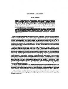
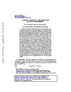
Figure 1. Structure of a typical triogram pseudo design matrix of Koenker and Mizera (2004) where gi is the pseudo design vector with elements gij = (Bj (xi , yi ))> , with Bj being a barycentric basis function, and hk the vector that represents the contribution of the k th edge of the triangulation to the total variation of the function in terms of the function values. The parameter λ is the smoothing parameter that controls the trade-off between fidelity to the data measured in the first term and roughness of the fit captured in the second summation. To express (14) as the regression quantile >  > .. > problem in (1), we introduce the (n + M) × n pseudo design matrix X = G .H


> > > ∈ Rn+M . where G = gi> , H = h> k , and the pseudo response vector y = z , 0 This can then be solved as the linear program in (3) or (4). Reverting back to the numerical analysis notations, the structure of a typical pseudo design matrix A> in (4) of the above triogram is presented in Figure 1. Figure 2 contains the pattern of the AQ−1 A> matrix. It is apparent from Figure 2 that the matrix to be factorized is extremely sparse. The portion of nonzero entries in AQ−1 A> is roughly 13/n. 5.1. Ng and Peyton’s Blocked Direct Solver. Separate timing of the four different steps in Ng and Peyton’s direct solver is presented in Figure 3. The amount of

Sparse Frisch Newton Algorithm

50

row 100

150

200

10

50

100 column

150

200

Figure 2. A typical AQ−1 A> matrix of the penalized triogram problem in Koenke rand Mizera (2004). time reported is the median execution time of solving the linear system of equations with AQ−1 A> as the coefficient matrix and the pseudo response vector in (14) as the right-hand-side in 50 replications of (13) for sample size ranges from 1000 to 50000. The rates of growth are reflected in the value of the least-squares slope coefficient b1 of the log-linear model fitted to the data points in Figure 3. The biggest chunk of time is expended in numerical factorization followed by minimum degree ordering. The fact that the nonzero pattern of the AQ−1 A> matrix remains unchanged from one iteration to the other enable us to perform the ordering and symbolic factorization steps only once over the whole iteration process in the Frisch-Newton algorithm. With a twenty-iteration execution, for example, an additional saving of roughly a factor of 1/5 in computing time can further be realized. 5.2. Sparse Frisch-Newton Algorithm. We perform a small scale simulation using the penalized triogram in (14) to fit the bivariate model in (13) to study the performance of our sparse implementation of the Frisch-Newton algorithm. We compare our sparse implementation (srqfn) to the implementation in Koenker and Mizera (2004), which utilizes the dense matrix version of the Frisch-Newton algorithm (rqfn) reported in Portnoy and Koenker (1997). Since it takes a long time for rqfn to solve the penalized triogram problem for just one replication for moderately large

Koenker and Ng

0.8

Symbolic Factorization

0.6 0.0

1000

5000

50000

1000

5000

50000

n

Numerical Factorization

Numerical Solution

0.6

10

n

b0 = −15.134 b1 = 1.332

0.4

Time

6

8

b0 = −15.2732 b1 = 1.582

0

0.0

2

0.2

4

Time

b0 = −13.5467 b1 = 1.1943

0.2

Time

b0 = −14.3633 b1 = 1.3709

0.4

0.0 0.5 1.0 1.5 2.0 2.5 3.0

Time

Minimum Degree Ordering

11

1000

5000 n

50000

1000

5000

50000

n

Figure 3. Median execution time (in seconds) of the four different steps in Ng and Peyton’s blocked left-looking sparse direct solver for sample size (in log-scale) ranges from 1,000 to 50,000.

size, we only perform 10 replications in the simulation study for n = 2(6 to 10 by 0.5) . Both implementations of the Frisch-Newton algorithm are coded in Fortran while the interfaces are in R. The simulation is performed on a Sun Sparcstation and the timings are clocked between the time the computation enters and leaves the Fortran code that performs the Frisch-Newton iterations, hence, eliminating any discrepancy on the overhead between the two implementations. Figure 4 reports the median execution time, in seconds, required to compute the triogram solutions. The advantage of srqfn over rqfn is obvious in Figure 4 over the whole range of sample sizes we have investigated. The factor of improvement ranges from roughly 36 at the sample size of 64 to approximately 850 at the sample size of 1024. Also reported in the legend of Figure 4 are the least-squares estimated coefficients of the log-linear model fitted to execution time on sample size. In Figure 5, we report the timing, in seconds, for only the srqfn for n = 2(6 to 14 by 0.5) . Also included in the figure are the least-squares estimated intercept and slope coefficients from regressing the log of execution time on the log of sample size. The estimated slope coefficient is almost identical to that in Figure 4, which suggests execution time grows exponentially at the rate of around 1.54.

Sparse Frisch Newton Algorithm

1e+04

12

rqfn: log(Time) = −11.49 + 2.53 log(n) srqfn: log(Time) = −11.16 + 1.51 log(n)

1e−02

1e+00

Time

1e+02

426

0.5

0.36

0.01

100

200

500

1000

n

Figure 4. Median execution time (in seconds) to obtain the penalized triogram solution to model (13) for rqfn and srqfn for sample size between 64 and 1024. Both axes are in log-scale. To compare the storage saving from our sparse implementation, we report in Figure 6 the memory requirement in bytes, needed to compute the penalized triogram solutions for different sample sizes on our Sun Sparcstation. What is evident from the figure is the quadratic increasing storage requirement of rqfn compared to the linear increase in srqfn.

Koenker and Ng

log(Time) = −10.92 + 1.54 log(n)

1e+02

srqfn:

13

1e+00 1e−02

1e−01

Time

1e+01

64.93

0.01 100

200

500

2000

5000

20000

n

Figure 5. Median execution time (in log-scale) of srqfn.

References Barrodale, I., and F. Roberts (1974): “Solution of an overdetermined system of equations in the `1 norm,” Communications of the ACM, 17, 319–320. Breiman, L., (1991). “The Π method for estimating multivariate functions from noisy data (Disc: 145-160)”, Technometrics, 33, 125-143. Duff, I.S., (1997). “Sparse numerical linear algebra: direct methods and preconditioning”, I.S. Duff, G.A. Watson (Eds.), The State of the Art in Numerical Analysis, Oxford University Press, Oxford, 27-62. Duff, I.S., (1998). “Matrix methods”, RAL-TR-1998-076, Department of Computation and Information, Rutherford Appleton Laboratory, Oxon. Duff, I.S., M.A. Heroux, and R. Pozo, (2002). “An overview of the sparse basic linear algebra subprograms: The new standard from the BLAS technical forum”, ACM Transactions on Mathematical Software, 28, 239-267. Friedman, J.H., (1991). “Multivariate adaptive regression splines (Disc: 67-141)”, The Annals of Statistics, 19, 1-67. Frisch, R., (1955). “The logarithmic potential method of convex programming”, Technical Report, University Institute of Economics, Oslo, Norway.

Sparse Frisch Newton Algorithm

14

1e+07 1e+05

Storage in Bytes

1e+09

rqfn: log(Storage) = 3.6 + 2 log(n) srqfn: log(Storage) = 7.5 + 1 log(n)

50

100

200

500

1000

5000

n

Figure 6. Storage requirement in bytes (log-scale) versus sample size (log-scale) for the rqfn and srqfn implementation when used to estimate the penalized triogram model.

Golub, H.G., and H.A. van der Vorst, (1997). “Closer to the solution: iterative linear solvers”, I.S. Duff and G.A. Watson (Eds.), The State of the Art in Numerical Analysis, Oxford University Press, Oxford, 63–92. Gonzaga, C., (1992). “Path-following methods for linear programming”, SIAM Review, 34, 167-224. Gu, C., D.M. Bates, Z. Chen, and G. Wahba, (1989). “The computation of generalized cross-validation functions through Householder tridiagonalization with applications to the fitting of interaction spline models”, SIAM Journal on Matrix Analysis and Applications, 10, 457-480. Gupta, A. (2002). “Recent advances in direct methods for solving unsymmetric sparse systems of linear equations”, ACM Trans. Math. Software, 28, 301-324. Hansen, M., C. Kooperberg, and S. Sardy, (1998). “Triogram models”, Journal of the American Statistical Association, 93, 101-119. Haunschmid, E.J., and C.W. Ueberhuber, (1999). “Direct Solvers for Sparse Systems”, Tech. Report AURORA TR1999-18, Vienna University of Technology. He, X., and P. Ng (1999): “COBS: qualitatively constrained smoothing via linear programming,” Computational Statistics, 14, 315–337.

Koenker and Ng

15

He, X., P. Ng and S. Portnoy (1998): “Bivariate Quantile Smoothing Splines,” J. Royal Stat. Soc., 60, 537–550. He, X. and P. Shi, (1996). “Bivariate tensor-product B-splines in a partly linear model”, Journal of Multivariate Analysis, 58, 162-181. Karmarker, N. (1984): “A new polynomial time algorithm for linear programming,” Combinatorica, 4, 373–395. Koenker, R. and I. Mizera, (2004). Penalized triograms: Total variation regularization for bivariate smoothing, Journal of the Royal Statistical Society (B), 66, 145–163. Koenker, R. and P. Ng, (2003). “SparseM: a sparse matrix package for R”, Journal of Statistical Software, 8, 2003. Koenker, R. and P. Ng, (2004). Inequality constrained quantile regression, manuscript. Koenker, R., P. Ng, and S. Portnoy (1994): “Quantile Smoothing Splines,” Biometrika, 81, 673–80. Koenker, R., and V. d’Orey (1987): “Computing Regression Quantiles,” Applied Statistics, 36, 383–393. Koenker, R., and V. d’Orey (1993): “A Remark on Computing Regression Quantiles,” Applied Statistics, 36, 383–393. Liu, J. W-H., (1985). “Modification of the minimum degree algorithm by multiple elimination”, ACM Trans. Math. Software, 11, 141-153. Lustig, I. J., R. E. Marsten, and D. F. Shanno (1992): “On implementing Mehrotra’s predictor-corrector interior-point method for linear programming”, SIAM Journal of Optimization, 2, 435-449. Lustig, I.J., R.E. Marsten and D.F. Shanno, (1994). “Interior point methods for linear programming: Computational state of the art”, ORSA Journal on Computing, 6, 1-14. Ng, E.G. and B.W. Peyton, (1993) “Block sparse Cholesky algorithms on advanced uniprocessor computers”, SIAM J. Sci. Comput., Volume 14, 1034-1056. Portnoy, S. and R. Koenker (1997). “The Gaussian hare and the Laplacian tortoise: computability of squared-error vs absolute error estimators”, (with discussions), Statistical Science, 12, 279-300. Saad, Y., (1994). Sparskit: A basic tool kit for sparse matrix computations; Version 2, available from: www.cs.umn.edu/Research/arpa/SPARSKIT/sparskit.html Saad, Y. and H. van der Vorst, (2000). “Iterative solution of linear systems in the 20-th century”, Journal of Computational and Applied Mathematics, 123, 1-33. Wright, S., (1997). Primal-Dual Interior-Point Methods, Society for Industrial and Applied Mathematics, Philadelphia. University of Illinois at Urbana-Champaign Northern Arizona University