Feb 1, 2008 -
JSS
Journal of Statistical Software February 2008, Volume 24, Issue 9.
http://www.jstatsoft.org/
A statnet Tutorial Steven M. Goodreau
Mark S. Handcock
David R. Hunter
University of Washington
University of Washington
Penn State University
Carter T. Butts
Martina Morris
University of California, Irvine
University of Washington
Abstract The statnet suite of R packages contains a wide range of functionality for the statistical analysis of social networks, including the implementation of exponential-family random graph (ERG) models. In this paper we illustrate some of the functionality of statnet through a tutorial analysis of a friendship network of 1,461 adolescents.
Keywords: relational data, social networks, exponential-family random graph models, statnet, R.
1. Introduction statnet comprises a suite of R (R Development Core Team 2007) packages for the analysis of social networks and other relational data. Previous papers in this issue describe in detail the functionality for most of these packages, and the underlying statistical theory behind it. In this paper we illustrate some of the functionality of three core packages within the statnet suite—network, sna, and ergm—through a tutorial-based analysis of a friendship network with 1,461 vertices. Readers of a more methodical nature may wish to examine the rest of the papers in this issue first. For those who do wish to tackle the tutorial early on, and who do not have much familiarity with statistical network models, we suggest that you begin by reading at least the introduction to this issue (Handcock, Hunter, Butts, Goodreau, and Morris 2008). In the tutorial, we assume a basic familiarity with R (including how to obtain further help or documentation for any of the commands we use) and with a variety of concepts and terminology from social network analysis. For newcomers, some of the latter may be understandable from context with the aid of a social network reference text, although those sections pertain-
2
A statnet Tutorial
ing to exponential-family random graph (ERG) models will likely require additional reading (Wasserman and Pattison 1996; Robins, Pattison, Kalish, and Lusher 2007a; Hunter, Handcock, Butts, Goodreau, and Morris 2008b). The statnet suite may be used to analyze a variety of types of network data from many different substantive domains, including directed and undirected, and one-mode and twomode (bipartite) networks. Some functionality also exists in the current version for handling dynamic networks and networks with missing data, both of which are undergoing continual development. However, for clarity, this tutorial will focus on a single dataset: a static, undirected, one-mode friendship network of 1,461 vertices. It is derived from data from the National Longitudinal Study of Adolescent Health, or Add Health (Udry 2003; Harris, Florey, Tabor, Bearman, Jones, and Udry 2003) by a process described in the Appendix. We call this dataset “Faux Magnolia High School”—Magnolia, because the schools on which it is based are large and located in the Southern US, and Faux because it is a model-based simulation from the original data, since the latter are subject to confidentiality restrictions. The data and analyses conducted in this tutorial are purposefully chosen to resemble those previously conducted by our group (Goodreau 2007; Hunter, Goodreau, and Handcock 2008a; Goodreau, Kitts, and Morris 2008). Throughout the tutorial, R input is represented by italicized typewriter font beginning with the R> prompt, or + prompt if it is a continuation of a previous line. Be sure to remove these symbols if copying and pasting commands into R. For convenience, all commands are also available in a standalone text file v24i09.R. Output from R is represented by regular typewriter font without these prompts, and we sometimes edit lengthy output and indicate deleted text using an ellipsis (...).
2. Obtaining the statnet suite of packages The packages in the statnet suite are connected via the meta-package statnet, which is little more than a wrapper for the other packages. To install and attach all packages, simply open R, and type: R> install.packages("statnet") R> library("statnet") Some users may only wish to obtain a subset of these packages. For this tutorial, only network, sna and ergm are required. One may install and attach each individually, although a shortcut is simply to install and attach ergm (which depends on network) and sna. Each of the individual packages mentioned here, along with the statnet package itself, is available from the Comprehensive R Archive Network (CRAN) at http://CRAN.R-project.org/. In addition, more information about the statnet packages is available on the Web at http: //statnetproject.org/.
3. License and citation information All statnet packages are free and open-source and are released under GPL (General Public License). The packages network and sna are released under GPL-2, while ergm is released
Journal of Statistical Software
3
under GPL-3 with attribution requirements for the source code and documentation. To obtain license information for all packages, simply type license.statnet(), or go to http: //statnetproject.org/attribution/. Please cite the statnet packages when you use them for research that is published or otherwise publicly distributed. Citation information is provided on our Web site at http:// statnetproject.org/citation.shtml, and can be obtained by typing citation("statnet"), or for any of the constituent packages by typing citation("").
4. Network exploration In this section, we explore methods for querying our data. We do not cover methods for importing, converting or manipulating network data; for information on these functionalities, please see Butts (2008a). To begin, make sure that the necessary packages are loaded into your current session (with library("statnet") or with both library("ergm") and library("sna")) and then load the dataset we will be analyzing, found in the ergm package: R> data("faux.magnolia.high") A shorter name will save us much typing effort: R> fmh fmh Network attributes: vertices = 1461 directed = FALSE hyper = FALSE loops = FALSE multiple = FALSE bipartite = FALSE total edges= 974 ... As this output is extensive (and includes the entire network edge list), it is often more useful to look at an abridged version of this information, which may be obtained by typing summary(fmh). Among other things, we see that the network has 1,461 vertices and 974 edges. Before we begin modeling these data statistically, it is good to have a general handle on their nature; perhaps the easiest way to do so for network data is by visualizing them. Since this is a large, sparse network, it is probably best to leave the isolates out:
4
A statnet Tutorial
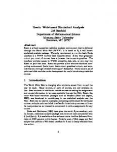
Figure 1: Faux Magnolia High, without isolates. R> plot(fmh, displayisolates = FALSE, vertex.cex = 0.7) Note that this command might take upwards of a minute or two, depending on the speed of your computer. There appears to be one large component and a smattering of many very small components (Figure 1), not to mention all of the components of size 1 that we removed from the visualization. To get a count of the component size distribution: R> table(component.dist(fmh)$csize) 1 524
2 64
3 29
4 11
5 12
6 4
7 7
8 4
9 1
11 1
12 1
19 1
23 439 1 1
From the output, we see that there are 524 isolates (which were not included in the visualization), one large component of 439 vertices, and many components in between. Let us look at an excerpt of the output given by the network summary: R> summary(fmh) ... Vertex attributes: vertex.names: Length Class Mode 1461 character character
Journal of Statistical Software
5
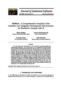
Figure 2: Faux Magnolia High, without isolates, colored by grade. Race: Asian Black 48 261
Hisp NatAm Other White 68 24 7 1053
Grade: 7 8 9 10 11 12 185 210 317 299 257 193 Sex: F M 768 693 There are four different vertex attributes associated with the vertices in this network: “vertex.names”, “Race”, “Sex”, and “Grade.” Grade is likely to be a strong determinant of social relations, so let us visualize the network with vertices colored by their grade: R> plot(fmh, displayisolates = FALSE, vertex.col = "Grade", vertex.cex = 0.7) Clearly there is a strong tendency for friendships to form within grade (Figure 2), although at the same time the grades themselves do not appear to be cohesive units; rather each grade seems to consist of a number of subgroups which link together. One might choose to explore other visualization options by typing help(plot.network). Network modelers are frequently interested in the degree distribution: R> fmh.degreedist fmh.degreedist
6 0 1 2 3 524 403 271 128
A statnet Tutorial 4 85
5 30
6 13
7 5
8 2
The cmode argument tells the degree command that since these are undirected data, we do not want to count both the upper and lower triangles of the sociomatrix, but rather only one. We could have chosen "outdegree" instead with identical results; leaving the argument off would yield numbers in the upper row double those seen above. The sna package provides individual functions for calculating a wide array of classic measures on networks, such as the previous command, degree. At the same time, the ergm package provides means for calculating any of the network statistics available for ERG modeling, all through the single command summary. For instance: R> summary(fmh ~ degree(0:8)) yields the same numerical results as the previous command from sna: degree0 degree1 degree2 degree3 degree4 degree5 degree6 degree7 degree8 524 403 271 128 85 30 13 5 2 Additional summary measures are available in both sna and ergm. Although there is some overlap in functionality, several functions remain unique within a package, so checking both for particular measures of interest may be helpful. A list of network statistics available for ERG models can be found in this issue (Morris, Handcock, and Hunter 2008); and for sna, in the package’s help files, via: R> help(package = "sna") One might also wish to compare degree distributions by sex: R> summary(fmh ~ degree(0:8, "Sex")) deg0.SexF deg1.SexF deg2.SexF deg3.SexF deg4.SexF deg5.SexF deg6.SexF 226 226 160 80 44 18 7 ... We leave it to the interested reader to split this out by sex, re-express as proportions and plot. Instead, we turn to another network feature that is commonly of interest, the count of triangles: R> summary(fmh ~ triangle) triangle 169 Instinct tells us that 169 triangles is many more than would be expected by chance in a network of 1,461 actors and 974 edges. We will revisit this in a more rigorous fashion below. Note that one can obtain more than one statistic at a time using this function; simply separate them with the plus symbol (standard syntax within R):
Journal of Statistical Software
7
R> summary(fmh ~ edges + triangle) edges triangle 974 169 When we visualized the network we saw a preponderance of within-grade edges. Let us display the mixing matrix by grade (i.e., the count of relationships cross-tabulated by the grades of the two actors involved): R> mixingmatrix(fmh, "Grade") Note: Marginal totals can be misleading for undirected mixing matrices. 7 8 9 10 11 12 7 110 11 3 3 0 0 8 11 165 9 7 0 2 9 3 9 152 24 10 4 10 3 7 24 151 38 11 11 0 0 10 38 152 32 12 0 2 4 11 32 90 Clearly most of the contacts are concentrated on the diagonal; you may wish to examine the mixing matrices for Race and Sex as well. To see a vector of attribute values for all of the actors for one of these attributes, or a table of the same, use the get.vertex.attribute command, or its shortcut, %v%: R> gr table(gr) 7 8 9 10 11 12 185 210 317 299 257 193 For more information on importing, exporting and manipulating network objects, see Butts (2008a) or the documentation for the network package. For more information on performing classical network analysis, see Butts (2008b) or the documentation for the sna package. Meanwhile, saving your work is always wise: R> save.image()
5. Fitting an ERG model The ergm package allows the user to fit exponential-family random graph (ERG) models to network data sets. These models, also known as p* (p-star), are described in great detail in earlier papers in this issue (Handcock et al. 2008; Hunter et al. 2008b), and elsewhere in the literature (Wasserman and Pattison 1996; Snijders, Pattison, Robins, and Handcock 2006;
8
A statnet Tutorial
Robins and Morris 2007). Very briefly, the model class formulates the probability of observing a set of network edges (and non-edges) as P(Y = y|X) = exp[θ T g(y, X)]/κ(θ), where Y is the (random) set of relations (edges and non-edges) in a network, y is a particular given set of relations, X is a matrix of attributes for the vertices in that network, g(y, X) is a vector of network statistics, θ is the vector of coefficients, and κ(θ) is a normalizing constant. Equivalently, the model states that the log-odds that any given edge will exist given the current state of the rest of the network is logit(Yij = 1) = θ T δ[g(y, X)]ij , where Yij is an actor pair in Y (which is ordered if Y is directed and unordered if not), and δ[g(y, X)]ij is the change in g(y, X) when the value of yij is toggled from 0 to 1. Let us begin with the simplest model of interest, a single-parameter model that posits an equal probability for all edges in the network. This model is known in different branches of network science as the Bernoulli model or the Erd¨os-R´enyi model, and it is a natural null model from which to proceed. In the ERG modeling framework, this corresponds to a model with a g(y, X) vector of statistics that contains only a single element, the number of edges in the network. R> model1 summary(model1) ========================== Summary of model fit ========================== Formula:
fmh ~ edges
Newton-Raphson iterations:
8
Maximum Likelihood Results: Estimate Std. Error MCMC s.e. p-value edges -6.99760 0.03205 NA