A Stochastic Parameter Approach - Ingenta Connect

ForestSm,nce,Vol 38, No 4, pp 825-841

Evaluatingthe Stabilityof Softwood Lumber DemandElasticityby End-Use Sector: A Stochastic

ParameterApproach DARIUS M. A•A•S

RoY BOYD

JOHNANGLE

ABSTRACT. Estimatesof the ehsticityof demandfor softwoodlumberare obtainedfrom a production

theoreticmodeldisaggregated by majorend-using sector.Modelparameters are treated as stochastic and estimatedusingthe Kalmanfilter algorithm.The analysissupports Spelter's(1985)earlierfindings of a highlyinelastic aggregate U.S. demandfor softwood lumberandthat thiselasticityhasdeclinedover the periodsince1950. The extentof the declinewas foundto be only some25%, however,andto haveoccurredin a relatively uniformfashion.Lumber demandelasticitiesin specificend-usesectorsvaried widely.

Significant declining elastidtytrendswerefoundonlyin residential upkeepandalteration andmaterialshandling. Thesetrendsarisefrombotha dec[ming shareof lumberin the costsof wood-based inputsanddeclining elasticities of demandfor the wood-based inputs themselves.At the aggregatelevel, the significant declining trendin elastidtyderives bothfrom changingconsumption sharesacrossend usesandfrom the combinedmovementsof the component elasticityseries.Foil. Scl. 38(4):825-841.

OFTWOOD LUMBER ISTHE LARGEST SINGLE CATEGORY OFFOREST PRODUCTS OUTPUT intheUnited States. Thuscharacteristics ofthedemand forsoft-

woodlumberare of specialinterestto bothprivateentrepreneursandpublic agencies in the forestsector.A keyelementin understanding the impactsof price changesor supplyshiftson softwoodlumberdemandis its ownpriceelasticity. Past studieshavegenerallyfoundthat lumberdemandis inelastic,but the range of availableestimatesis broad (0.0 to -0.88). More recently, Spelter (1985) examinedlumberdemandonanend-usebasis,concluding thataggregatedemand elasticityis in the lowerend of the rangefoundin earlierstudies(-0.11 in 1980) andthatthe elasticityhasdeclinedin a trendfashionby asmuchastwo-thirdsover the post-WWlIperiod.Giventhisarrayof empiricalestimates,andthe potential existenceof trendsin lumberdemandelasticity,further studyseemswarranted to providesomeclarification for policyanalysis. The presentpaperreexamineslumberdemandby end usewith specificattention to its potentialvariationover time. We beginwith a brief review of past lumber demandstudiesand critiqueof Spelter'sapproach.We show that the functionalform usedby Spelterleadsto end-usedemandehsticitiesthat decline in a fairly predictablefashion.Economictheory suggests,however,that agents

NOVEMBER 1992/825

may alter their behaviorin a varietyof ways in responseto technological and

policychangesfi Thus,afterderiving ourtheoretical model,we employ a stochasticcoeffidentsapproach,the Kalmanfalter,that allowsdemandparameters, including the own-priceelasticity,to vary freelyovertime.

As notedabove,paststudiesof U.S. softwoodlumberdemandhaveproduceda

widerangeof pointestimates for own-price demand elasticity. •' All haveused fixedcoefficients modelsandfunctional formsyieldingeitherconstantelasticities or linearmodelswhere(short-term)elasticityvariesonlyas the price-quantity equilibrium shifts.Most haveexaminedsoftwoodlumberas a composite thougha few have distinguished speciesgroups(e.g., Douglas-fir,southernpine). Only three [Cardellichio and Veltkamp(1981), Rockeland Buongiorno(1982), and

Spelter(1985)]havedisaggregated demand by end-usesector?The demand specification in most studiesderivesdirectlyfrom traditionalmicroproduction theory, either in an ad hoc fashionor by direct derivationfrom a costfunction. Technological changein the production processes employing lumber,whereit has beenconsidered, hasusuallybeenrepresented by a simpletimeproxy.Adjustment dynamics,due to costs,expectations, or institutional rigidities,havebeen representedby somevariantof the partialadjustment processor someexplicit distributedlag in pastprices. An importantexception to allbutthe fixedcoefficients condition is the studyby Spelter (1985), which examinesinput substitutionin lumber end uses in the context of explidt processesof technological adoptionderived from diffusion theory.In contrastto otherstudies,Spelter'smodelentailselasticitychangesas the diffusionprocessproceeds.Thus, for the period1950 to 1980, he findsthat the own-priceelasticityof demandfor the aggregateof all softwoodlumberfell from - 0.285 to - 0.111.

The existenceandtime patternof the elasticitydeclineare, however,essentiallyguaranteed by the form of Spelter'smodel.For any givenend use, i, and time period,t, demandis givenby the inverselogarithmicfunction:

Ot•/Mt•= Ui[1 - K,exp(-b•/Tti)]

(1)

where

Or/is the quantityof lumberdemanded

Mt• is the levelof end-useoutput • For a detailed explanation of thistypeof behavior andtheproblem it presents for econometric modelers, see Lucas (1976).

2 Thereappear tobeninepublished studies sincethemid-190)s thathavegivenexplicit estimates of lumberdemandelastidty(pointestimatesshownin squarebracketsfor all softwood lumberunless otherwisenoted):Adamsand Blackwell(1973) [0]; Adams(1977) [0]; Mills andManthy(1974)

[-0.02 for "structuralspedes"];McKillopet al. (1980) [-0.17]; Spelter(1985) [-0.285 to -0.111]; Waggener et al. (1978)[-0.35]; Robinson (1974)[ -0.88 for Douglas-fir species]; Rockel andBuongiorno (1982)[-0.91 for residential construction enduse];andMcKillop(1967)[-3.2].

3 Baudin andSolberg (1989)present analternative approach toanalysis ofdemand byendusewith application to the Norwegianlumbermarket.

826/FOP, m't'SCnmCE

Ui is the maximumpotentialuse of lumberper unit of end-useoutput(a parameterto be estimatedin most cases)

Tti = Tt- i,i + (P(e)it- P(n)i•)/P(n)it, thecumulative percentage pricechange P(e)itis the "in-place" priceof the existinglumber-using technology P(n)itis the in-placepriceof some"new"technology bi > 0 and1 •> Ki > 0 are parameters to be estimated

Changes overtimein theelastidtyof OtwithrespecttoPL dependonthesignof the term b - 2T(1 - Kexp(-b/T)). For T < b/[2(1 - Kexp(-b/T))], this ehsticitywill rise as T risesandfor T > b/[2(1 - Kexp(- b/T))] it will fall (T is the percentprice changecumulatedover time). The valuesof b andK are estimatedfromdatain a givenenduseandhencethe pointat whichelastidtytrends changeis data dependent.Oncethis pointis passed,however,the ehsticity cannotrise over time so long as T continuesto increase,as it does over the historicaldata samplefor all of the end usestreated in this form in Spelter's analysis. Further,the functional formguarantees thatthe elasticitywilldeclineat a decreasing rate overtime: fallingrapidlyat firstfor smallervaluesof T, aswould obtainin the earlyportionsof the sampleperiod,andlessrapidlyas T increases. Thisbehaviorcanbe seenin Figure2 of Spelter's(1985)paper.

Giventhat Spelter'sresultsdependheavilyon the specificform of his demand function,further analysisof the existenceand form of trends in lumberdemand

ehstidty seemsjustified.We developour modelfrom basicconsiderations of microproduction theory.Production in eachend-useis viewedas involving the combination of an array of compositeor aggregateinputs(Chambers1988)-Spelter's"technologies." Thesegoodsare comprised of morebasicinputs(lumber, plywood,steel, labor, energy, etc.) produced,we assume,under fixed proportionstechnologies. We identifytwo specificcomposites,one that uses lumber(IL) andone(Io), a substitute, thatdoesnot. The remaining composites (e.g., in the caseof residential construction thesemightincludeplumbing, electrical,painting, grading, etc.) andthepairlz andIo areassumed separable. Thus the production function for a particular end-use(0e) couldbe writtenas:

O, = f(g(IL,Io), h(I• I i, ...)) whereI• Ip . . . areothercomposite inputs.

(2)

If producersare costminimizers,andgiventhe separability assumption, the conditional demand for thelumber-using (composite) inputwilldependonlyonthe pricesof the composite inputsin the functiong in (2) andoutput.That is, IL = ILOVXL, Pxo, O,)

(3)

For thisdualityto holdbetweenweaklyseparable production andweaklyseparablecostfunctions (andconditional factordemands) the aggregator function, g, mustbe homothetic. We assume thattheproducers ofthecomposite inputsI L andIo (whichmaybe the samefirmsas the producers of 0,) are alsocostminimizers. Sinceoutputof the composites is fixedproportions, asassumed, theirproduction functions canbe

NOVEMBER1992/827

writtenasIz. = min{kz.L,kwW,. . .} andIo = min{doO,dwW,. . .}, whereL

islumber, Wislabor,0 isothermaterials, etc.,andtheki anddjareconstants. The costfunction forIL outputisthenC*(Pz.,Pw..... Iz.) = (Pz./k•. + Pw/kw+ ß ß .)/z.wherepz.,Pw,Po are pricesof lumber,labor,andothermaterials[see,for example,Chambers (1088,p. 59-60)].P•z.andP•o,asusedin (3), arethengiven byP•z.= Pz./k•.+ Pw/kw+ ßßßandP•o= Po/do+ Pw/d•+ . . . (themarginal costsofIL andIo), andtheconditional demand forL is oC*/Op•. = L = (1/kz.)I•.. Combining thislastexpression with(3), andimposing homogeneity ofdegreezero in factorprices,yields:

Z = (1/kL)IL(P•L/P•o, Oe)

(4)

For the presentanalysiswe assumethat g in (2) canbe representedby a Cobb-Douglas technology withconstant returnsto scale.We allowfor the prospectof technological changewithing by incorporation of a timetrend.Fromthese assumptions and(4) the lumberdemandequationcanbe writtenas:

ln(L/OOit= aoit+ alitln(P•L/P•o)it + a2itlnt

(5)

Finally, to approximatethe adjustmentdynamicsof demand,we assumethat producersbase their purchasesof lumberon expectedrequirementsfor the

currentyear,(L/Oe)*io andlastyear'sactualactivity,(L/Oe)i,t-•,sothat:

In(L/Qe)i,t = •i,t In(L/Qe)*i,t q- (1 - •i,t)In(L/Oe)i,t-1

(6)

wherefn-ms set%,tbetween 0 and1 basedontheirconfidence oftherealization of (L/OO*i,t;the lattergivenby Equation (5). Thisis thefamiliar partialadjust-

mentmodel. 4 Substituting Equation (5)into(6)andrearranging termsyields the lumber end-use demand function:

In(Z/Oe)it = bo,i,t + bl,'gJn(PIL/Plo)i,t + b2,i, thlt+ ba,i, thl(Z/Oe)i,t-1 + •i,t (7) where

(L/OOi, t is termedthe "end-use factor" bi.i. t = %,taj. i.tforj = 1, 2; ba,i, t = 1 - •i,t •i.t is therandom errortermfor theith endusein thetthperiod.

Short-run effects aregivenbythebj.i.ttermswhilelong-run effects arecalculated

asai.i.t= bi,i.t/%,t = bi.i.t/(1 - bs, i,t)for/ = 1, 2.s Equation(7) formsthe generalbasisfor ourempirical analysis. It is essential to recognize,however,thatthe adjustment processneednotbe the sameacrossall end-use categories. Construction applications mayinvolvethelongest lagsinlight of buildingcodelimitations, unionlaboragreements,etc., whileusesin manufacturingor residential upkeepandalteration mayadaptmorerapidlysincethereare fewerinstitutional barriersto change.In our empirical analysis we employstatisticalteststo checkfor properspecification of the adjustment structure. NeitherP•z. nor P•o includeestimatesof capitalcostsnor do we includea measureof capitalstockin g as mightbe appropriate if capitalwere viewedas quasi-fixed.In some cases, such as residentialconstruction(see Rockel and Guj2r2ti (1988,pp. 520-521)showsthatthepartialadjustment modeldoesnotintroduce serial correhtioninto the error term as do someotherdistributed hg models.

Thelongrunehstidties actually change eachperiod, buttheycanbeinterpreted asthelongrun elastidtywhichwouldexistceterisparibus.

828/FO•-srscm•qCE

Buonglorno1982) andresidentialupkeepandalteration(wherea largevolumeof lumberis soldfor do-it-yourself application), capitalcostsmaybe relativelysmall. In other uses, suchas manufacturing, the end-useindustryis so large andheterogeneous that a meaningful measureof capitalcostsor stockas associated with the lumberinputis unavailable. Thus,we believethatit is reasonable to assume, as do RockelandBuonglorno(1982) in the caseof residentialconstruction alone, thatcapitalandnoncapital inputsare stronglyseparable in the end-useproduction processes.

The Cobb-Douglas specification assumedfor g in (3) yieldsa convenient form for estimationbut carrieswith it the assumptions of constantreturnsto scaleand unitelasticityof substitution. Its useis notwithoutsupportin pastempirical work, however.DoranandWilliams(1982)andGellner,Constantino, andPercy (1989), in studiesof demandfor forestproductsin construction, employthe generalized Leonfiefcostfunction(consistentwith CRS and CES in the underlyingtechnology) in whichthe conditional factordemandrelationsare a linearversionof (6). Also Rockel and Buongiorno(1982) in a study of forest productsdemandin residentialconstruction foundthe generalizedCobb-Douglas form the mostappropriatecostfunctionspecification andestimatedreturnsto scaleof 1.018. The costminimization specification impliesthat end-useoutputis exogenous. Though this assumptionis seldomjustifiedin empiricalstudiesof the forest productssector,it maybe quitereasonable for the construction andresidential upkeepusesof lumber.Foliain(1979) characterizes the construction industryas comprising manyfirmsof similar(small)sizewithlow capitalrequirements.Under theseconditions, it is commonto observemarketquantitiesestablished by consumers(demand)while producersset price. Empiricalestimatesof the price elasticityof construction supplyby bothFollain(1979)andMontgomery(1989) showno statistically significant quantityresponse.Sincethe residentialupkeep and alteration componentof lumber demandinvolvesmuch the same market structureit may alsobe reasonable to view thissectoras operatingwith output fixedby demandas well. For the remainingend-usesectors(materialshandling and"other,"thelatterbeingprimarilymanufacturing uses)theassumption of fixed sectoroutputis lessobviously applicable. We retainit here becauseof the difficultyof identifying a reasonable outputpricemeasurefor thesehighlyaggregated end-uses.

A finalconcernrelatesto the treatmentof factorpricesas exogenous in the estimation process.Few forestsectorstudies,employing eitherthe costor profit function approach, consider the problems of potentialsimultaneous determination of the forestproduct,laborandotherpricesusedin factordemandrelations.In the presentanalysis,the end-useindustriescovervirtuallythe entire economy, suggesting thatnearlyallfactorpricesbe replacedby someinstrument(inlimited informationestimation).Given the problemsencounteredin earlier studieswith

the useof largenumbers of instruments 6 andthe experimental natureof our application of the Kalmanfilter, we have electednot to use instruments. 6 Theresidential construction costfunction studybyRockelandBuongiorno (1982)isoneofthefew examples wheresuchproblems havebeenaddressed. Theirattemptsto replaceallfactorpriceswith instnnnents leadto problems of wrongsignsandhighvariances for estimatedcoefficients, whichwas thoughtto arisefromtheincreased collinearity oftheinstnnnents. Asa consequence theyretainedthe OLS approach.

NOVEMBER 1992/829

Estimationof Equation(7) requiresinformation on lumberconsumption by endusecategory,end-useoutput,andthe factorpricescomprising the two composite inputsPxL and Pxo. For the period 1950 through1987, we collectedand/or computeddata for eachof these variablesin five end-usecategoriesas listed belowwith their associated end-useoutputmeasure. End-usecategory Residentialconstruction (single,multi-family

Outputmeasure Floor area of all units started

and mobile units) Nonresidential construction

Realvalueof nonresidential construction put-in-

Residentialupkeepand improvement

place Real valueof upkeepandalterationexpendi-

Materialshandling(pallets,dunnage,crating,

Realvalueof manufacturing shipments

turesin "lumber-using" activities ? etc.)

"Other" (all manufacturing, nonresidential upkeep and repair, etc.).

Indexof manufacturing production

Estimatesof lumberconsumption by end-usecategorywere derivedfrom infermarionpublished by WesternWoodProductsAssociation (1989)andprovidedby

Spelter. 8 Computation of composite inputpricesfollows theapproach described by Spelter(1985)for hisP(e) andP(n) termswiththe following exceptions: (1) Pr/• andPro for residential construction are composites ofthe costsfor sheathing and sidingon a per housingunit basis; (2) Pr/• in materialshandlingis a weightedcompositeof the producerprice indexof softwoodlumberandan indexof wagesin SIC 42 (transportation services),Pro is a composite of the priceindexof paperboard andSIC 42 wages;and (3) Pr/• in "other"is the priceindexof softwood lumberwhilePro is the simpleaverage of the priceindexof softwoodplywoodandthe all commodity producerpriceindex.

A summarydescription of dataconstruction methodsis givenin the appendix.

The lumber demandfunctionswere estimatedusing the "Kalmanfilter" ap-

preach. øVarious stochastic coefficient methods havebeenusedineconomic research, includingthose developedby Hildreth and Heuck (1968), Cooley and Prescott (1976), and Swamy and Tinsley (1980). We have used the "Kalman Filter" methodbecauseit is the most generalof these approaches in that it 7 "Lumber-using" activities withinthe Department of Commerce reportsonresidential upkeepand alterationweredefinedasincluding siding,remodeling, and"other"categories andexcluded plumbing, painting,andheating,whichwouldnot normallyinvolvemuchuseof lumber.

8 Tabulations developed by HenrySpelter,USDA,ForestService,ForestProducts Laboratory, Madison,Wisconsin.

9 Descriptions of the Kalmanfilterapproach canbe foundin Kalman(1960),KalmanandBucy (1961), Harvey and Phillips(1982), NewboldandBos (1985), andJudgeet al. (1985). A detailed discussion of the generalityof the Kalmanfilter approachis availablein Harvey (1990).

830/FOms'rscw-•CE

0.5

RES NRES

-0.5

-1

•OTHER -1.5

1950

I

I

I

1960

1970

1980

--

1990

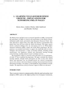
FIGUI• 1. Kalmanfiltercoeffidentestimatesfor priceterm by end-use(RES, residential; NRES, nonresidential; RUA, residential upkeepandalteration; MH, materialhandling; OTHER, other uses).

assumesthe leastaboutthe underlyingstatisticalstructureof the time varying processandgivesbackthe mostinformation abouthowthatprocessevolvesover time.lO

We initiatedthe estimationprocedurewith ordinaryleast squares(eLS) regressions whichwe examined for serialcorrelation andspecification bias.Durbin's h (Durbin 1970) indicatedautocorrelation problemsonly in the nonresidential constructionend use. ] tests (Davidsonand MacKinnon1981) were used to examinealternativespecifications of the demandfunctionsandled us to eliminate the trend variablefromthe equationsfor all five end-usesectors.This cannotbe construedas a conclusive test for the absenceof technicalchangeandmay only reflectthe inadequacy of a simpletimetrendasa representation ofactualtechnical shifts.In addition,trendwiseandmorecomplexformsof technical changemaybe capturedin the variationof individual coefficients. We thenemployedthe Kalman algorithm,allowingthe coefficientsto vary over time. eLS and Kalmanfilter coefficient estimatesare shownin Table1 togetherwith regression diagnostics. AnnualKalmanfiltercoefficient estimates are plottedin Figurei andassociated lumberpriceelasticityestimatesin Figure2 (togetherwith simpletime trend regressions).The Kalmanfilter estimatesshownin Table 1 are the meanvalues •oIn thecourse of thisresearch weconsidered aswelltheHildreth-Houch (H-H)approach, specifically thevariantproposed bySinghet al. (1976).Withthismethod,significant timevariation forthe relativepriceparameter wasfoundonlyin the residential construction andresidential upkeepand alterationsectors.Resultsfor the residentialsectorare suspect,however,becausesomeof the estimates of the variances of the randomcomponent of parameterfluctuation were negativedespite useofH-H'sfour-step estimation procedure. Thesewerearbitrarily settozero,asH-H suggest, with uncertain impacton the finaltimevaryingestimates.Discounting the residential construction result, thisis the samesectoralpatternof timevariationfoundwiththe Kaitaartfilterapproach.

NOVEMBER1992/831

RF•SIDENTIALUPKEEPANDALTERATION

RESIDENTIAL CON•TRUCBON

OTHER

TOTAL SOFTWOOD LUMBER

O2

0

FIGUP. E 2. Elasticitiesof demandfor softwoodlumberby end use: Kalmanfilter resultsandcomparisonwith Spelter(dottedlinesare lineartrendsfor Kalmanfilter values).

for the estimationsample.Their standarderrors are usefulin indicatingwhether the coefficients are relativelystableor unstable,butare not sousefulfor indicating statisticalsignificance. The smallsamplepropertiesof asymptotict milos com-

putedfrom these standarderrors in the usualmannerare unknownand they shouldonlybe viewedas suggestive. The goodness-of-fit test for the Kalmanfilter equations is a likelihoodratiotest whichteststhe nullhypothesisthat there is no significant differencebetweenthe fixedcoefficients OLS equationandthe Kalmanfilterequations. The test statistic is L = - 2(LR - L u) whereL is the log-likelihood ratioto be tested,LR is the log-likelihood functionof the (restricted)OLS equation,and Lu is the loglikelihoodfunctionof the (unrestricted)Kalmanfilter equations.L is asymptoti-

callydistributed asa X2 statistic withdegrees of freedom equalto oneplusthe number oftimevarying coeffidents intheoriginal modeltimesthree.n Thus,for the residentialconstructionsectorwith two time-varyingparametersthere are 7

degreesof freedomwhilethe "other"sectorhasonlyonetime-varying coefficient and hence4 degreesof freedom. RESIDENTIALCONSTRUCTION

Annualvaluesof the Kalmanfilter estimatesfor the lumberpriceterm for residenilalconstructionin Figure 1 displayno consistenttrend and only limitedvari-

ation.TheX2testsupports thenullhypothesis thatthefixedcoefficients model is appropriate. Annualelasildtyestimates plottedin Figure2 showlittletrendapart n Eachtime varyingcoeffidentin the originalmodelis associated withthreeparameters in the Kalmanfilter analysis:a time varyingcoeffident,a transientcoefficient,anda variance.The error variancefor the equationas a wholemustalsobe directlyestimatedandso comprises an additional parameter.

832/FOhSSTSC•CE

NOVEMBER 1992/833

from extreme initial and terminalvalues. The simpletrend regressionis not significantat the 0.05 level. These results are at variancewith Spelter's (1985) findingsin whichall residentialconstructionend-usecategorieswere foundto have significant,positive diffusion parameters(- bi in Equation(1) is negativeas requiredfor a mature goodfacinga declining market shareandfallingdemandelasticity).Our sample averageelasticityestimates( - 0.13 in the shorttermand - 0.55 in the longterm) are alsomuchlower than RockelandBuongiorno's (1982) resultsof -0.91 for softwoodlumberdemandin residentialconstruction. Spelter, unfortunately,did not report elasticitiesby end-usecategory. NONRESIDENTIAL CONSTRUCTION

OLS estimates for nonresidential construction are corrected for first-order autocorrelation since the Durbin h statistic based on initial OLS results indicated the

presenceof serialcorrelation.Equivalence of the OLS andKalmanfilter results cannotbe rejected basedon the likelihoodratio test, and there is no variationin the annualKalmancoefficients in Figure 1. Annualelasticityestimatesare three to four timeslargerthanthosefoundfor residentialconstruction, andthe average long-termelasticityis -1.15. The annualestimatesshow no significanttime trend.

Spelter's(1985) analysis,in effect,reachesthe sameconclusion with regardto the absenceof elasticity•ends. The singleindependentdiffusioncoefficientreportedamonghisfourcategoriesof nonresidential construction is positivebut not significantly differentfrom zero. RESIDENTIAL UPKEEP AND ALTERATION

Softwoodlumberconsumption per unit of residentialupkeepand alterationexpenditureincreaseddramatically relativeto trendlevelsin the 1978-1982period. This shiftwas likely due to risinghousingpricesandmortgagerates whichlead consumersto forgo new home purchasesand turn to repair and remodelingof existingstructures.Sinceour modeldoesnot considerthe broaderconsumer decisionof "moveup" versusrenovationof the existingdwelling,we introducea dummyvariablewhichtakeson a valueof 1 for the periodfrom 1978 to 1982. The explanatory powerof the OLS regressionis significantly lowerthanin the two previousconstruction sectors.Spelter(1985)encountered thissameproblem

(hereports anR2of0.39fora sample period from1950through 1981)andpoints to the highdegreeof variabilityof lumberconsumption in thisenduse. Because of the statisticalinsignificance of the laggedendogenousvariable,it was subse-

quentlydroppedfromour modelspecification. The Kalmanfilter resultsfor this secondspecification confirmthe instability of lumberdemandin residential upkeep andalteration.AnnualKalmanfilter estimatesshownin Figure1 fluctuatemore than thosefor residentialconstruction and exhibita gradualdecliningtrend (in absolutevalue)over the sample.The L statisticrejectsthe nullhypothesisof no differencebetweenthe OLS andKalmanfilter modelsat the 5% levelof significanca.

Annualelasticityestimatesin Figure 2 displaythe instabilityof underlying coefficients.The simple time trend, hoveever,is significantat the 0.01 level.

834/FOmS•ct•cE

Spelter (1985) also estimateda significant,positivediffusionparameterfor this enduse, but foundit necessaryto augmenthisstandardspecification throughthe inclusionof a real per capitaincometenn. MATERIALS HANDLING

In the OLS regressionfor the materialshandlingsector,a 4-year movingaverage

of the priceterm capturedthe priceeffectmuchbetter thanthe simplecurrent value.This, in turn, impliesthat the dynamiceffectof priceis morecomplicated in thismarket--risingto a peakafter3 yearsandthendeclining exponentially. The demandrelationin this sectorseemsto be quitestable.Equalityof the OLS and Kalmanfilter resultscouldnot be rejectedonthe basisof the likelihoodratiotest, andthe Kalmanprice term showsno variationin Figure 1. The plot of lumber price elasticityestimatesin Figure 2, however, does suggestsome declining trend--the simpletrend beingsignificant at the 0.01 level. Spelter's(1985)resultsin thisenduseare mixed.In hisanalysisthe materials handlingcategoryis splitinto two groups:palletsand shipping.He founda significant,positivediffusion coefficient for the shipping groupbut nopricesensitivity in pallets.Over the time spanof ouranalysis,softwoodlumberusein palletsrose from an insignificant level in the 1950s to a volume more than twice that of shipping in the 1980s.Shipping,in contrast,declinedsteadilyas an endusefrom 1950through1987.Theseoffsettingtrendsmaybe reflectedin the stabilityof our pricecoefficient for the aggregatesector. OTHER USES

The "other"end-usecategoryis a heterogeneous aggregation of lumberapplications,includinga substantialcomponentof residualerror from poormeasurement of consumption in the otherfourcategories.As a resultit is highlyvolatileandnot readilymodeled.In our initialregressionsnoneof the coefficients of Equation(7) were significant. After testsof alternativespecifications, we deletedall variables excepta simple4-yearmovingaverageof the pricetenn. Our Kalman filter results indicate that this sector too has been unstable over

time. The likelihoodratio test rejectsthe nullhypothesisof stability.The coeffident valuesin Figure1 revealno systematictrendin the pricevariable,but seem to fluctuaterandomlyaroundthe meancoefficientvalueof -0.6345. This is also evidentin the plot of elasticityestimatesin Figure 2, whichhas an insignificant simpletime trend. Our "other" categorycombinesthe furniture, other manufacturing, railroad ties, and"other"groupingsusedby Spelter(1985). Of thesegroupings,Spelter took furnitureas exogenous,"other" was representedas a fractionof consumptionin the "defined"usesandmodeledas a functionof softwoodlumberprice and a time trend, and onlythe railroadties groupingwas foundto have a significant diffusion coefficient.

The elasticityof demandfor lumberdependsonthe characteristics of demandfor the lumber-using commodityandof the production technology in whichlumberis

NOVEMBER 1992/ 835

employed.For a two-factor,competitive,ORSindustry,Hicks(1963) hasshown that the ehsticityof demandfor one of the factorsdependson the ehsticityof substitution betweenthe factors,the elasticityof demandfor the productusing the factors,the ehsticityof supplyof the other factor, andthe factor'ssharein totalcosts(or productgivenORS).Hicksshowsthatthe elasticityof demandfor the factormovesdirectlywith eachof these determinants. Sincewe assumethatthe supplyof allfactorsis perfectlyelasticandthat the elasticityof substitution betweenfactorsis zero in the composite inputs,Hicks' originalformuhtionconvergesto e = kd where e is the elasticityof (derived) demandfor lumber,k is the shareof lumberin total costsof I•., andd is the (negative of) elasticityof demand for theproduct,I•.. The elasticityof demand for I•. wouldbe foundfrom its (conditional) demandfunctionin Equation(3). Given

ourassumption of fixedproportions production forI•, however, d = bl,i,t from the estimationEquation(7). The share of lumberin total cost, usingearlier notation,wouldbe k = (pffk•.)/(pffk•.+ P•/kw). ThusHick'srehtionsimplifies to:

e = kd = (pffk•.)/(pffk•. + Pw/kw)bl,i, t

(8)

Direct derivationfrom Equation(7), of course,yieldsthe sameresult. The elas-

ticityof demand for lumberwillfallif its sharein thecostsofproducing I•. fallsor if the demandehsticityfor I•. itselffalls.The formercouldoccurif, over time, lumberprice(PD roselessrapidlythanthepriceof the otherinput(Pw)or if k•.

rises rehtive tokw.22Adecline inthedemand ehstidty forI•. implies shifts inthe parametersof the underlying(Cobb-Doughs) production functiong in (2). From our empiricalanalysis,the constantcoefficients(OLS) modelscan be rejectedonlyfor the residentialupkeepandalterationandotherend-usesectors. Of thesetwo, only the upkeepandalterationresultshowsany evidenceof a

consistent trendin thepricecoeffident (b•,i.t)overtime(seeFigure1). In our simplifiedCobb-Douglas production context,this impliesno changein the basic productiontechnology--theehsticitiesof outputwith respectto the two compositeinputshavebeen constant--forthe residential,nonresidential, andmaterials handlingsectors.The large reductionsin lumberuse per unit of end-use outputobservedoverthe sampleperiodin thesesectorswere, by thesefindings,

occasioned entirelyby changes in relativepricesof the composites andnot by shiftsin the technologyof production.There is somelimitedevidencein other studiesto supporttheseconclusions. RockelandBuongiorno (1982)founda small but significantly positivesignfor the time trendtechnology proxyin their conditionallumberdemandfunctionfor residential construction. They arguethatthis may reflect improvements in housingquality;but it doesappearthat "other influences" swampwhatevertechnicalchangeeffectsmighthavebeencaptured by the time trend. Also, to the extent that productionmethodsare similarin NorwayandtheUnitedStates,the BaudinandSolberg(1989)studyofNorwegian lumberdemandprovidessomeevidencefor hck of technical changein thebuilding andconstruction sectors;time trendswere foundto be significant onlyin the prefabricatedhousingsector. In upkeepandalteration,however,our resultsgivesomeevidenceof technical 12In thepresent analysis, however, wehaveheldthetechnical coefficients intheproduction ofIL constant.

836/FOmSUScm•cE

change.In this sector,at givenrelativefactorprices,factorintensityhasshifted towardthe nonlumber input.Thismayhavebeenduebothto the emergenceand rapidgrowthof the do-it-yourself marketfor homerepairs(wherepanelproducts are muchpreferredto lumber)andto the risingimportance of additions(which involvemore materialsinputsof all types)relativeto repairs. All of the end-uselumberdemandelasticitiesshownin Figure2 have some downwardtime trend. However, onlythosefor residentialupkeepandalteration and materialshandlingare significantlydifferentfrom zero (at the 0.05 level) in simpletime trend regressions.For residentialupkeepand alteration,the time pattern of the cost shareterm (k) complements that of the compositeinput demandelasticity.For materialshandling,the elasticitytrend derives entirely from a declinein the relative share of lumberin the cost of the lumber-using compositefactor. If the softwood lumber consumed in the five end-use sectors is assumed to be

homogeneous in quality,the total demandfor lumbercanbe obtainedby simple summationof the demandcurvesfor each end use, and the elasticityof this aggregatedemandfunctionis the averageof the elasticities for the five enduses weightedby their respectivesharesof total consumption. This seriesis shownin the finalpanelof Figure2, togetherwith a plotof Spelter'sreportedresultsfor the sampleperioddecadepoints.The Kalmanfilterresultshowsa distincttimetrend whichis significant (at the 0.01 level)in a simpletimetrendregression. Giventhe lackof significant trendsin mostof the enduses,thisoutcomemaybe thoughtto turnprimarilyon the changing shares(weights)of the endusesin totalconsumption. But this appearsto be onlypart of the cause.A declining patterncontinues to emergewhen end-useelastidtiesare weightedby constantsharesor are unweightedin a simpleaverage.These alternateseriesshowtrendsthat are significant(at the 0.01 level) in simpletrend regressions,but do not declineas rapidlyasthe seriesin Figure2. Thusthe fallingtrendin the aggregate seriesin Figure2 is dueas well to the variouslycomplementary andcounterposing movements in the elastidties of the constituent end-use series.

The totallumberKalmanfilter seriesin Figure2 showsa roughlylineardecline over time in contrastto the inverseJ-shapeof Spelter'smodel.We haveargued abovethat the form of the latter is largelydictatedby use of the redprocal logarithmic functionin the diffusion model.Over the periodfromthe mid-1950sto the mid-1980s,the Kalmanelastidtiesfall by roughly25% (Spelter'sestimates declineby 50%) andin 1980are (on trend)35% higherthanSpelter'sestimate. A final concernrelates to the dynamicresponseof the aggregatedemand elasticity.Becausepricesare incorporated in Spelter'smodelin the form of a cumulative percentage difference variable[T• in Equation(1)], a sustained lumber pricechangeceteris paribusleadsto gradually cumulating quantityresponses over time. In our modelthese adjustmentsderivefrom the laggedpriceanddemand quantityterms. To abstractfromthe absolutedifferences in elasticityestimates betweenthe two approaches, Figure3 compares elasticityadjustments relativeto

short-term levelsforseveral historical timepoints?After4 years,ouranalysis showsan increasein elasticityof roughly 1.75-2.0 times the short-term level while Spelterfoundnearlya three-foldexpansion.Our modelalsofindsa much

ValuesforSpelter's modelwerescaled fromhisFigure6.

NOVrMSrS 1992/837

ELASTICITY{t+n)/ELASTICITY (t) 3.5

2.5

1.5

K]: 1960

0.5

KF 1985

ß

I

0

1

0

KF 1970

.......

KF 1980

SPELTER 1950

.......

SPELTER 1970

I

2

3

PERIOD (n) FIGURE 3.

Adjustment of total softwood lumberdemandelasticityover time (ratiosrelativeto zero lag)fromKabnanfilter modelandSpelter(1985)for variousyears.

larger differencein the dynamicresponsebetweenthe earlierandlater yearsof the sampleperiod. In sum, our analysisconfirmsfindingsby McKillopet al. (1980), Mills and Manthy (1974), Spelter (1985) and othersof a highlyinelasticaggregateU.S. demandfor softwoodlumber over the post-WWlI period. It also supports Spelter'sconclusion that this elasticityhasdeclinedover the periodsince1950. We findthe extentof the decline,however,to be onlyabout25% over the past 3 decadesandto haveoccurredin a relativelyuniformfashion.Lumberdemand elasticitiesin specificend-usesectorsappearto vary widely. We were able to identifysignificant declining elasticitytrendsonlyin residentialupkeepandalterationand materialshandling.In the contextof our model, these trends can be attributedbothto a decliningshareof lumberin the costsof wood-based inputs andto declining elastidtiesof demandfor the wood-based inputsthemselves.At the aggregatelevel, the decliningtrendin elasticityderivesbothfrom changing consumption sharesacrossend usesandfrom the combinedmovementsof the componentelasticityseries.

ADAMS,D.M. 1977. Effectsof nationalforesttimberharveston softwoodstumpage,lumber,and plywoodmarkets--aneconometric analysis.OregonStateUniv. For. Res. Lab., Res. Bull. 15. Corvallis,OR. S0 p.

ADAMs,F.G., andJ. BLACKWELL. 1973. An econometric modelof the UnitedStatesforestproducts industry.For. Sci. 19(2):82-96.

838/FoR•rscm•cE

BAUDIN,A., and B. SOLBERG. 1989. Substitutionin demandbetween sawnwoodand other wood

productsin Norway.For. Sci. 35(3):692-707. CARDELLIC•IIO, P., andJ.J.VELTKAMP. 1981.Demandfor PacificNorthwesttimberandtimberproducts,studymoduleIIA. Reportto thePacificNorthwestRegionalCommission, Vancouver,WA. CHAMBERS, R.G. 1988.Appliedproduction analysis:A dualapproach. Cambridge Univ. Press,New York. 331 p.

COOLEY, T.F., andE.C. PRESCOTT. 1976. Estimationin the presenceof stochastic parametervariation. Econometrica 44:167-184.

DAVIDSON, R., andJ. MAcKn•NON. 1981. Severaltests for modelspecification in the presenceof alternativehypotheses.Econometrica 49:781-793. DORA•,H.E., andD.F. WILLIAMS. 1982. The demandfor domestically-produced sawntimber:An application of the Diewertcostfunction.Aust.J. Agric.Econ.26(2):131-150. DURI•IN, J. 1970.Testingfor serialcorrelation in least-squares regression whensomeof the regressorsare laggeddependent variables.Econometrica 38:410-421. FOLLAn% J.R. 1979.The priceelastidtyof the longrun supplyof new housing construction. Land Econ. 55(2):190-199.

GELLNER, B., L. CONSTANT•NO, andM. PRRC¾. 1989.Dynamicadjustments in the U.S. andCanadian construction industries. Econ.BranchWork.Pap.ForestryCanada,Economics Branch,Ottawa, Ontario,Canada.23 p. GUJARATI, D.N. 1988. Basiceconometrics. Ed. 2. McGraw-Hill,New York. HARVEY, A.C. 1990. Forecasting,structuraltime seriesmodelsand the Kalmanfilter. Cambridge Univ. Press, New York. 556 p.

HARVEY, A.C., andG. PHILLIPS. 1982.Estimation ofregression modelswithtimevaryingparameters. P. 306-321in Games,economic dynamics andtimeseriesanalysis, in Destier,M., E. Furst,and G. Schwodianer (eds.). Physica-Verlag, Wien-Wurzburg. HIcKs,J.R. 1963. The theoryof wages.St. Martin'sPress,New York. 247 p. H•LDR•Ti•,C., andJ.P. HOUCK.1968.Someestimatorsfor a randomcoefficient regression model.J. Am. Star. Assoc. LXIII:584-595.

HOGG,R.V., andA.T. CRAIG.1978.Introduction to mathematical statistics.Ed. 4. Macmillan,New York. 437 p. JUDGE, G.G., STAL.1985.The theoryandpracticeof econometrics. Ed. 2. Wiley,New York. 1019p. KALMAN,R.E. 1960. A new approachto linear filteringand predictionproblems.J. BasicEng. 82:34-45.

KALMAN, R.E., andR.S. BucY.1961.New resultsto linearfilteringandpredictiontheory.J. Basic Eng. 83:95-107. LUCAS, R. 1976. Econometric policyevaluation: A critique.P. 19-46 in The PhillipsCurveandthe labormarket,supplement to J. MonetaryEcon.

McKILLOP, W. 1967.Supplyanddemand for forestproducts: Aneconomic study.Hilgardia 38:1-132. McKILLOP, W., T.W. STUART, andP.J. GEISSLER. 1980. Competition betweenwoodproductsand substitutestructuralproducts:An econometricanalysis.For. Sci. 26:134-148.

M•LLS,T.J., andR.S. MANTHY. 1974.An econometric analysis of marketfactorsdetermining supply anddemandfor softwood lumber.MichiganStateUniv.Agric.Exp. Stn. Res. Rep. 238 p. MONTGOMERY, C.A. 1989. Longrunsupplyanddemandof new residentialconstruction in the United States:1986to 2040. USDA For. Serv. Res. Pap. PNW-RP-412.39p. NEWBOLD, P., andT. Bos. 198S.Stochastic parameterregression modelsseries:Quantitative applicationsin the socialsciences.SagePublications, BeverlyHills, CA. ROBINSON, V.L. 1974. An econometric modelof softwoodlumberandstumpage markets.For. Sci. 20:171-179.

ROCKEL, M.L., andJ. BUONGIORNO. 1982. Deriveddemandfor woodandother inputsin residential construction: A costfunctionapproach. For. Sci. 28(2):207-219.

SINOH,B., A.L. NAGAR, N.K. CHOUNDRY, andB. RAI.1976. On the estimation of structuralchange: A generalization of the randomcoefficients regression model.Internat.Econ.Rev. 17(2):340361.

NOVEMBER1992/839

SPELTER, H. 1985. A productdiffusionapproachto modelingsoftwoodlumberdemand.For. Sd. 31:685-700.

Sw•l¾, P.A.V.B., andP.A. T•NSLE¾. 1980.Linearprediction andestimation methodsfor regression modelswith stationarycoefficients. J. Econ. 12:103-142. W^C•ENER,T.R., G.F. SC•P,•UDER, and H.M. HO•SON.

1978. Elastidties of demandfor forest

productsover time. Inst. For. Resour.Rep. Univ. of Washington, Seattle,WA. WESTERN WOODPRODUCTS ASSOCIATION. (Variousissues).Statistical yearbookof the westernlumber industry.Portland,OR. Copyright1992by the Sodetyof AmericanForesters ManuscriptreceivedJuly 16, 1991

DariusM. Adamsis withthe Schoolof Forestry,Universityof Montana,Missoula,MT 59812-1063; RoyBoydis withthe Economics Department,OhioUniversity,Athens,OH 45701;andJohnAngleis withtheEconomic Research Service/U.S.D.A.,1301New YorkAvenue,Washington, DC 20001.The authorswouldlike to thankTheodoreBos, RogerConway,JanKmenta,andVishwaShuklafor their helpfulcomments duringthe variousstagesof thisresearch.

ResidentialConstruction (PricesperHousingUnit) Pit = (100*PPI(SL) + 18*CARPWAGES)*lFAMSIZE Plo = (90*PPI(SP) + 9*CARPWAGES)*IFAMSIZE where

PPI(SL) = producerprice indexfor softwoodlumber

PPI(SP) = producerpriceindexfor softwoodplywood CARPWAGES = carpenterwages

1FAMSIZE= average floorareaof single familyhousein 1000ft2 Theserelationsare Spelter's(1985)formulasfor sheathing andsidingon a per house basis.

Residential Upkeep andAlteration (Prices per1000ft2 ofFloorArea) Pit = (100*PPI(SL) + 18*CARPWAGES Plo = (100*PPI(SP) + 10*CARPWAGES)*0.9

Theserelationsderivedfrom Spelter'sformulasfor residentialupkeepandalteration.

NonresidentialConstruction (PricesperJob) P•L = 0.75*(0.7*PPI(SL) + O.I*CARPWAGES) + 0.25*(PPI(SL) + 5*CARPWAGES)

P•o = 0.75*(0.6*PPI(METAL) + O.05*CARPWAGES) + 0.25*0.9*(PPI(SP) + 4*CARPWAGES)

840/FOmS•SCIF.•CE

where

PPI(METAL) = producerpriceindexfor metalproducts.

Theserelationsderivedfrom Spelter'sformulasfor nonresidential buildings. MaterialsHandling

P•L = 0.25*PPI(SL) + 0.75*TRANSWAGES P•o = 0.9*PPI(PB) + O.i*TRANSWAGES where

PPI(PB) = producerpriceindexfor paperboard

TRANSWAGES = indexof wagesin SIC 42 (motorfreighttransportandwarehousing) Other

PiL/Pio = PPI(SL)/(O.5*PPI(SP) + 0.5*PPI(ALL)) where

PPI(ALL) = all commodityproducerprice index

NOVEMBER 1992/ 841