A Stochastic Programming Approach to Improve ... - University of Alberta

A Stochastic Programming Approach to Improve Overbooking in Clinic Appointment Scheduling

Michele Samorani Leeds School of Business, University of Colorado at Boulder, UCB 419, Boulder, Colorado 80309-0419, {[email protected]}

Linda LaGanga Mental Health Center of Denver, 4141 East Dickenson Place, Denver, Colorado 80222 {[email protected]}

Overbooking by scheduling appointments beyond capacity is a common way to reduce the negative effect of no-shows in outpatient clinic settings. Recent works have considered the show probability of individual patients in order to improve scheduling by increasing provider utilization and patient access to healthcare services.

In this paper, we define a stochastic

program that finds the optimal schedule given an estimate of the actual show probabilities of a set of patients. We study the effect of the estimation accuracy and of the number of scenarios used on the clinic profit. Our results show that, although the clinic profit increases with the number of scenarios considered, only one scenario is sufficient to achieve significantly higher profit than that obtained by scheduling the patients randomly.

Samorani and LaGanga — 2

Keywords: Appointment Scheduling, No-shows, Overbooking, Stochastic Programming, Healthcare Last Revision: 2/20/2011 .

1. Introduction Appropriate clinic scheduling is important in meeting healthcare demand (Green and Savin, 2008; Gupta and Denton, 2008).

Patient no-shows are a realistic consideration in clinic

operations (Kaandorp and Koole, 2007), where they reduce clinic productivity (LaGanga and Lawrence, 2007b) and cause revenue shortfalls (Kim and Giachetti, 2006; Moore, WilsonWitherspoon, and Probst, 2001). Appointment scheduling techniques to address these problems include allocating capacity for open access through short-term and same-day scheduling (Kopach et al., 2007; Liu, Ziya, and Kulkarni, 2010; Qu et al., 2007; Robinson and Chen, 2010), and overbooking to mitigate the effects of patient no-shows (LaGanga and Lawrence, 2007b). Recently, Glowacka et al. (2009), Muthuraman and Lawley (2008), and Zeng et al. (2009) have considered the show probabilities of individual patients, as opposed to the global show rate considered in previous works. This enhancement improves scheduling performance by, for example, avoiding an empty first slot of the day to reduce provider idle times, and scheduling low show-probability patients towards the end of the day to reduce clinic overtime. However, these models present a few drawbacks. First, their overbooking model assigns multiple patients to the same slot, whereas it has been shown that overbooking by reducing the time between appointments, as in LaGanga and Lawrence (2007b), is preferred (LaGanga and Lawrence, 2007a) to prevent long patient wait times. Second, to exploit the knowledge of individual


probabilities, the models assume exponential service times (Muthuraman and Lawley 2008, Zeng et al. 2009) or use a greedy scheduling algorithm that often finds suboptimal solutions, such as the one proposed by Glowacka et al. (2009), who schedule patients in order of their show probabilities. We overcome both drawbacks by using a stochastic programming model that finds the optimal schedule by using the slot compression technique. Our mathematical formulation aims at maximizing the clinic utility function as defined by LaGanga and Lawrence (2007b) to account for the benefits of serving more patients balanced with the costs of patient wait time in the clinic and overtime costs, which are incurred when extra patients show up because overbooking is used. Our model’s input consists of the individual show probabilities of the patients to be scheduled, and the output is an assignment of the patients to the slots. We test our method by repeatedly scheduling sets of patients with randomly generated show probabilities. Our results indicate that it is sufficient to use only one scenario to obtain a schedule that is significantly better than a random scheduling – this is equivalent to rounding the show probabilities to 0 or 1; even better results (although not significantly better) can be obtained by considering more scenarios (i.e. a better approximation of the probabilities), but this increases the computational times. In Section 2, we formally introduce the mathematical problem and the stochastic programming model. Section 3 reports our experimental results. In Section 4, we draw some conclusions on our approach, highlight its benefits and drawbacks, and identify future research directions.


2. Mathematical Formulation LaGanga and Lawrence (2007b) introduced the approach of overbooking by slot compression to increase clinic productivity and the number of patients served. Suppose that the goal is to schedule a subset of

patients in the slots of a certain day. Furthermore, suppose that each

appointment has a constant length

and that the clinic capacity is equal to

session starts at time 0 and ends at time patients at times 0,

,

, …,

, i.e. the clinic

. Without overbooking, the clinic would schedule ; but, with overbooking, the clinic uses

, in such a way that patients are scheduled every

slots, with

time units.

Table 1. Notation

Duration of an appointment Interval between scheduled appointments, Number of patients to schedule Clinic capacity, i.e. the number of appointments obtained by setting

Number of appointments scheduled (i.e. number of slots), Profit for scheduling a showing visit request Cost for each unit of patient waiting time Cost for each unit of clinic overtime


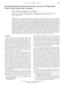
Figure 1 represents this form of overbooking, in the case of

. The lower part of the

figure reports the patients scheduled if overbooking is not used (patients are scheduled every time units); the upper part reports the patients scheduled if overbooking is adopted (patients are scheduled every T time units).

x1

x2

x3

x1

x4

x2

x5 x3

x6 x4

Figure 1. The effect of overbooking by slot compression

The advantage of overbooking is obviously to increase the number of patients seen. On the other hand, this technique possibly introduces waiting time and overtime when extra patients show up.

The objective is to find the optimal trade-off among the following conflicting

objectives: 1) Maximize the number of patient shows 2) Minimize the patients’ waiting time 3) Minimize clinic overtime The weight of these objectives is determined by the values of ,

, and

(see Table 1). The

objective function is therefore to maximize the overbooking utility function: ∑

Where

is 1 if patient

scheduled in slot ,

will show,

∑

∑

is the binary variable that indicates if patient

is

is the continuous variable representing the waiting time of the patient


scheduled in slot , and waiting patient

is the continuous variable representing the overtime. Note that each

contributes to the overall waiting time cost with a term

. We use this

strategy to establish consistent units of measurement for the costs of patient wait time and clinic overtime. In order to define the stochastic program, we need to answer the following question: if we knew which patients will show and which ones won’t, in which slots should they be scheduled? Let us introduce a few definitions that will help to solve this problem: : scheduled initial time of the -th slot; : actual finish time of the visit of the patient assigned to the -th slot; : earliest initial time of the patient assigned to the -th slot, i.e., the time when the appointment scheduled in slot can begin. It is equal to the maximum between the scheduled initial time for the patient and the finish time of the (

)-th slot;

: waiting time experienced by the patient scheduled in the -th slot. If the patient does not show, it must be equal to 0; otherwise, it is equal to

, the difference between the

finishing time of the previous appointment and the scheduled initial time of the -th appointment.

are given and equal to (0, , 2 , …); the values of

The values of the

,

, and

can be

computed recursively as follows:

∑ equal to

(i.e. otherwise)

is equal to 0 if no showing patient is scheduled in the first slot; it is


{

}

∑ ∑

{

It is obviously possible to include the expression for

∑

{

inside the one for

:

};

Note that the finishing time for slot j is equal to the earliest initial time if the patient assigned to j does not show, otherwise it is equal to the earliest initial time plus the length of the appointment . The optimal schedule is found by solving the following mathematical model for the clinic profit function:

∑

∑

∑

(1)

s.t.

(

∑

)

(2a) (2b)

∑

(3a)

∑

(3b)


∑

(3c) (4)

∑

(5)

∑

(6) {

}

Constraints (2a) and (2b) implement the recursive definition of waiting time, as defined above. Similarly, constraints (3a), (3b), and (3c) implement the recursive definition of finishing time. Constraints (4) defines the overtime as the difference between the finishing time corresponding to the last slot and the scheduled finishing time

. Constraint (5) makes sure that each patient

is assigned to at most one slot; similarly, (6) guarantees that at most one patient is assigned to each slot. The model (1)-(6) can be used only if we know which patients will show and which won’t. Let us explain how to apply the concepts seen above to the case where we know only the show probabilities of the patients. Consider

patients, each having a show probability

We define a stochastic program based on a set of scenarios

as the set of all

elements. Although the total number of scenarios is | |

consider only the set of the most likely scenarios

).

, where each scenario

corresponds to the set of the showing patients. Therefore, we can denote possible subsets of

(

, let us

, otherwise solving the problem would

be impractical. The model (1)-(6) can then be extended to the case of many scenarios. In this


model, the objective is to maximize the expected overbooking utility function. We still have the binary decision variables

, which are equal to 1 if and only if patient i is assigned to slot j. On

the other hand, the earliest starting times, finishing times, waiting times, and overtime are all referred to a scenario . Let us introduce the following variables:

: the waiting time experienced by the patient scheduled in slot j under scenario S : the finishing time of slot j under scenario S : the overtime experiences under scenario S

Furthermore, let us denote with

the probability of realization of scenario S, and with

scalar that is equal to 1 if patient i shows in scenario

and 0 otherwise. Thus, the model

develops as follows:

∑

[ ∑

∑

]

(7)

s.t.

(

∑

)

a

(8a) (8b)

∑

(9a)

∑

(9b)

∑

(9c) (10)


∑

(11)

∑

(12) {

}

The task of finding the set

of most likely scenarios can be performed by enumerating the

scenarios from the most likely to the least likely, until the probability covered by the scenarios in is large enough. For example, suppose that the show probabilities are 0.1]. In the following discussion, the expressions “patient

[0.98, 0.6, 0.2,

” and “probability

equivalently, in the sense that a patient is identified by his/her probability

” are used

. A “branch-and-

bound” tree is built in order to enumerate the most likely scenarios in decreasing order of probability. In this context, each node n is associated with 3 sets patients that have been “fixed” as shows (

̅,

while the sets

̅

and

̅

,

. They contain the

), the ones that have been fixed as no-shows (

and the ones that are available because they have not been fixed ( are in set

,

). At the root ̅, all patients

are empty. This means that, at this stage, no patient has

been fixed to show or no-show. Each node

is also characterized by an upper bound

is equal to the probability of the highest-probability scenario that is reachable from .

∏

),

∏

∏

{

}

, which


In our example, the highest probability scenario reachable from the root is the one where show, while

and

do not show. The reason is simply that

being therefore more likely to show, while

and

and

and

are greater than 0.5,

are smaller than 0.5, being therefore more

likely not to show. The upper bound at the root is:

{

}

{

}

At each node , two child nodes and moving him/her to

and

and

{

}

{

}

are generated by choosing one patient in A

, respectively. In other words, two nodes are generated by fixing

an available patient to show or not. After a node is generated, the upper bound Suppose, for example, that patient

is computed.

is chosen to branch from the root ̅. The two child nodes

have the following characteristics:

{

̅

{

{

From

̅

{ },

},

̅

,

̅

,

̅

{

}

{

}

{ },

̅

{

}

{

}

} {

̅

},

̅

}

̅ , all scenarios where

shows can be generated. Among them, the one with the

highest probability has probability 0.106. From

̅ , all scenarios where

does not show can

be generated. Among them, the one with the highest probability has probability 0.423. Since we are interested in enumerating the scenarios sorted by decreasing probability of realization, the node chosen to branch is the one with the highest upper bound. At the -th level


of the tree,

is empty, and therefore the scenario is identified by the patients in set

;

furthermore, the probability of realization of the scenario is given by the value of the upper bound. The number of scenarios generated is limited by a parameter , which we call “scenario coverage”: scenarios are generated until a probability greater than of their probabilities. If

is covered by the summation

is set to 0, only the most likely scenario is generated. This situation

corresponds to rounding the show probabilities of the patients to 0 or 1. If, on the other hand, is set to 1, this corresponds to generate all

scenarios.

3. Experiments Let us consider a clinic that adopts overbooking by slot compression. We assume that the show rate is , the capacity of the clinic is has a constant length for example, if

= 10, the number of slots is

= 1. Therefore,

= 60 minutes,

= 13, and each appointment

. This value of

can be impractical;

would be equal to 46’10’’. Nevertheless, since we study the

impact of classification accuracy and number of scenarios on the clinic performance, we disregard this issue. The other parameter values are fixed at values of

and

,

,

. The

are the ones chosen by LaGanga and Lawrence (2007b), while the value of

that we choose is smaller (0.15 instead of 0.50). The reason is that the waiting time term included in the objective function of LaGanga and Lawrence (2007b) is the average waiting time experienced by showing patients; in this paper, as mentioned in section 2, we use the consistent cost units of total wait time and overtime. Therefore, we must choose a smaller value for

, in

order not to overestimate the waiting time cost. The tests consist in scheduling

patients using their actual individual show probability

or an estimation of it. We assess the impact of the accuracy of this estimation, which we call


“estimation accuracy”, because this indicates how much time should be spent to optimize the prediction of the individual show probabilities. We assess how many scenarios (in the form of the scenario coverage ) should be included in the model in order to obtain satisfactory results. The procedure we use in our tests is depicted in Figure 2.

Input: Show rate s, Estimation accuracy w, Scenario Coverage 1. Randomly generate the

patients as follows:

a. Let A be the Beta Distribution where

,

. The expected

value of A is s. This is the distribution used to sample the actual show probabilities. b. Sample

from A.

is the actual show probability of the patient.

c. Let E be the Beta Distribution where value of E is

,

. The expected

. This is the distribution used to sample the predicted

show probability of the current patient. d. Sample

from E.

is the predicted show probability of the patient

2. Generate the minimum number of scenarios that covers . 3. Solve the stochastic program (6-10) to find the optimal scheduling 4. Compute the clinic profit, the total waiting time, and the overtime Figure 2. Test Procedure

In step 1, we generate probability

patients by randomly sampling their individual actual show

and the their individual estimated show probability

.

The actual show


probability is used to determine if the patient shows or not; the estimated show probability represents the output of a hypothetical classifier which tries to predict if the patient shows or not. Although the typical output of a classifier is simply the predicted class (show or no-show), the basic output of most classification techniques is “a numeric value that represents the degree to which an instance is a member of a class” (Fawcett 2006), which can be promptly transformed into the probability of belonging to each class. In steps 1a and 1b, we assume that the real show probability of each patient follows a Beta distribution A, with parameters expected value is s. To this end, we fix

and we compute

and

, whose

. The value of

has

been fixed to 1, so that the probabilities are evenly spread across the interval [0, 1]. Figure 3 shows the probability density function for = 0.7.

Figure 3. Probability function for beta distribution A, in the case = 0.7

The estimated probability

, computed in steps 1c and 1d, is sampled from another Beta

distribution E, with parameters a function of

and

. As for distribution A, the value of

is computed as

; but, unlike for distribution A, the expected value of E should be equal to

.


To this end, the value of

is computed as

. The deviation from the expected value

depends on the estimation accuracy, which is represented by the parameter : 1.2 (low accuracy), 2, 5, 106 (perfect accuracy, i.e.

4 values of

the probability distributions for each value of

. We consider

). Figures 4a-d show

, assuming that the actual show probability

is

equal to 0.7.

Figure 4a. E distribution for

Figure 4c. E distribution for

Figure 4b. E distribution for

Figure 4d. E distribution for

In step 2 of the procedure, we generate enough scenarios to reach a predefined scenario coverage

= 0.0 (i.e. only one scenario), 0.1, 0.2, 0.3, or 0.4. We limit our analysis to these

cases because, for P > 0.4, the solution time can be very large. In step 3, the problem is solved with a 2-minute time limit and with a tolerance gap of 3%. In other words, the solution method is stopped either if 2 minutes have passed or if a solution is found whose value is less than 3%


apart from the current upper bound. After the optimal scheduling has been found (step 4), the actual individual show probabilities are considered to determine which patients show, and, therefore, the values of the clinic profit, the waiting time, and the overtime. The testing procedure of Figure 2 is executed 100 times for each show rate for each

= 0.0, 0.1, 0.2, 0.3, 0.4, and for each

= 0.6, 0.7, 0.8,

= 1.2, 2, 5, 106. We used the same random

seed to generate the patients throughout the 100 repetitions, so that they have the same characteristics

and

for each parameter combination. Tables 2-4 report the average clinic

profit for each show rate, compared to the clinic profit obtained by randomly assigning the patients to the slots.

Table 2. Average clinic profit for Show Rate = 0.6 Show Rate = 0.6 Random 0.00

7.07

7.00

7.00

7.06

6.90

0.10

6.94

7.02

7.09

7.08

6.90

0.20

7.08

7.05

7.14

7.12

6.90

0.30

7.05

7.05

7.12

7.10

6.90

0.40

7.07

7.17

7.17

7.14

6.90

Table 3. Average clinic profit for Show Rate = 0.7 Show Rate = 0.7 Random 0.00

7.68

7.73

7.71

7.75

7.53

0.10

7.74

7.72

7.84

7.90

7.53

0.20

7.70

7.81

7.77

7.92

7.53

0.30

7.75

7.81

7.85

7.85

7.53

0.40

7.80

7.83

7.87

7.92

7.53

Table 4. Average clinic profit for Show Rate = 0.8


Show Rate = 0.8 Random 0.00

7.93

7.99

7.91

7.94

7.71

0.10

7.95

8.00

7.99

7.98

7.71

0.20

8.06

7.96

7.88

7.96

7.71

0.30

7.97

8.05

8.05

8.01

7.71

0.40

8.01

8.02

8.04

8.10

7.71

As expected, Tables 2-4 suggest that the clinic profit is positively correlated to the scenario coverage

and to the estimation accuracy

values of

> 0, because, for

. The correlation with

is more evident for

= 0, the predicted show probabilities are simply rounded to 0 or 1,

which makes any two predictions equivalent, unless one is below 0.5 and the other above 0.5. Interestingly, the clinic profit is significantly larger than the one achieved by a random scheduling policy even for paired t-test with

= 0. For each combination of

and

, we performed a one-tailed

in order to compare the average clinic profit obtained when

= 0 to

the one obtained by the random scheduling policy, and underlined in Tables 2-4 the cases where = 0 achieves a significantly larger profit than random scheduling. This happens in 9 out of 12 cases. Similarly, for each combination of

and

, we performed 4 one-tailed paired t-tests with

in order to compare the clinic profit obtained by 0.40, to the one obtained by using many scenarios (

= 0.10,

= 0.20,

= 0.30, and

=

=0. This second set of tests aims at assessing the advantage of ) rather than just one (

). The cases when a value of

greater

than 0 obtains a significantly larger clinic profit are highlighted in bold in Tables 2-4. Surprisingly, this happens only 4 times out of 48 t-tests. Obviously, it would happen more often if larger values of

were considered.

Table 5 reports the computation time needed for solving the stochastic problem (7)-(12). Clearly, it is larger for larger values of , because of the explosion of the number of scenarios.


Note that, without the 2 minute time-out, the average computation times would probably be much larger.

Table 6 reports the frequency, as percentage, of the runs where a time-out

occurred. Note that, for

, it happens in more than 10% of the runs. It is therefore clear

that this method becomes impractical for larger values of .

Table 5. Average computation times (seconds) for each show rate and scenario coverage. Show rate 0.60

0.05

0.58

6.22

13.96

25.32

0.70

0.06

0.71

5.63

17.36

34.05

0.80

0.05

0.39

4.69

11.38

21.92

Table 6. Frequency (%) of time-outs for each show rate and scenario coverage. Show rate 0.60

0.00 %

0.00 %

2.75 %

6.75 %

13.00 %

0.70

0.00 %

0.00 %

1.50 %

6.75 %

17.50 %

0.80

0.00 %

0.00 %

1.50 %

4.75 %

10.00 %

.

4. Conclusions In this paper, we considered the problem of scheduling patients in the presence of no-shows, using the technique of overbooking by slot compression proposed by LaGanga and Lawrence (2007b).

Assuming that an estimate of the individual show probabilities is available, we

proposed a stochastic model to find the scheduling that maximizes the clinic profit, defined as a weighted function of the number of showing patients, clinic overtime, and patient waiting time. We studied the performance of our method on sets of randomly generated patients, and compared its performance to the one obtained by randomly scheduling the patients.


Our experiments show that it is sufficient to consider only one scenario in order to achieve a significantly larger clinic profit than the one obtained by the random scheduling policy. In other words, instead of considering the individual show probability, one could just consider a binary prediction (i.e., show or no-show) for each patient. Furthermore, our experiments suggest that an even larger profit can be obtained by considering more scenarios, but the improvement upon the single-scenario case would be significant only if the number of scenarios was very large (e.g. ), but this would make our method very slow. This finding suggests that, in spite of all existing work that is founded on individual show probabilities, decision makers could just use a simple binary classifier based on whether a patient is more likely to show up or not. This simple consideration can simplify the implementation of appointment scheduling systems, and, ultimately, can lead to a vaster adoption of overbooking in real world applications to increase clinic profit. Our work has two major limitations. First, we assume that show probabilities and their estimates follow a Beta distribution, which may be not accurate. In other words, we use artificial data and a predefined distribution to generate the predictions, while the most correct approach would be to consider a real world dataset and a real classification technique. In future work, we use real data and perform more testing of the data distribution and real data mining classification techniques. The second limitation is that our methodology, which uses a stochastic program to solve this problem, is very efficient if only one scenario is considered; but, as the number of scenarios increases, the computational times explode. Possibly, it may be more efficient to use a solution method based on Approximate Dynamic Programming (Powell 2007), where a slot is assigned to a patient at each stage.


References Fawcett, T. 2006. An introduction to ROC analysis. Pattern Recogn. Lett. 27(8) 861-874.

Glowacka, K.J., R.M. Henry, J.H. May. 2009. A hybrid data mining/simulation approach for modeling outpatient no-shows in clinic scheduling. Journal of the Operational Research Society. 60 1056 –1068.

Green, L.V., S. Savin. 2008. Reducing delays for medical appointments: A queuing approach. Operations Research. 56(6) 1526 – 1538.

Gupta, D., B. Denton. 2008. Appointment scheduling in health care: Challenges and opportunities. IIE Transactions 40 (9), 800 – 819.

Kaandorp, G. C., G. Koole. 2007. Optimal outpatient appointment scheduling. Health Care Management Science 10(3) 217 – 229.

Kim, S., R.E. Giachetti. 2006. A stochastic mathematical appointment overbooking model for healthcare providers to improve profits. IEEE Transactions on Systems, Man, and Cybernetics – Part A: Systems and Humans 36(6) 1211 – 1219.

Kopach, R., P.C. DeLaurentis, M. Lawley, K. Muthuraman, L. Ozsen, R. Rardin, H. Wan, P. Intrevado, X. Qu, D. Willis. 2007. Effects of clinical characteristics on successful open access scheduling. Health Care Management Science 10(2) 111 – 124.


LaGanga, L.R., Lawrence, S. R. (2007a). Appointment scheduling with overbooking to mitigate productivity loss from no-shows. Proceedings of Decision Sciences Institute Annual Conference, Phoenix, Arizona, November 17-20, 2007.

LaGanga, L. R., Lawrence, S. R. (2007b). Clinic overbooking to improve patient access and increase provider productivity. Decision Sciences 38(2) 251-276.

Liu, N., S. Ziya, V.G. Kulkarni. 2010. Dynamic scheduling of outpatient appointments under patient no-Shows and cancellations. Manufacturing & Service Operations Management 12(2) 347 – 364.

Moore, C. G., P. Wilson-Witherspoon, J.C. Probst. 2001. Time and money: Effects of no-shows at a family practice residency clinic. Fam. Med. 33(7) 522 – 527.

Muthuraman, K., M. Lawley. 2008. A stochastic overbooking model for outpatient clinical scheduling with no-shows. IIE Transactions 40, 820-837.

Powell, W.B. 2007. Approximate Dynamic Programming: Solving the curses of dimensionality. Hoboken, NJ: John Wiley and Sons, Inc.


Qu, X., R.L. Rardin, J.A. Williams, D.R. Willis. 2007. Matching daily healthcare provider capacity to demand in advanced access scheduling systems. European Journal of Operations Research 183(2) 812 – 826.

Robinson, L.W., R.R. Chen. 2010. A Comparison of Traditional and Open-Access Policies for Appointment Scheduling. Manufacturing & Service Operations Management 12(2) 330 – 346.

Witten, I. H., E. Frank. 2005. Data mining : practical machine learning tools and techniques, Morgan Kaufmann series in data management systems. Amsterdam; Boston, MA: Morgan Kaufman.

Zeng, B., A. Turkcan, J. Lin, M. Lawley. 2009. Clinic scheduling models with overbooking for patients with heterogeneous no-show probabilities. Annals of Operations Research 178(1) 121 – 144.