A Structured and Unstructured grid Relocatable ocean ... - CyberLeninka

Deep-Sea Research II ∎ (∎∎∎∎) ∎∎∎–∎∎∎

Contents lists available at ScienceDirect

Deep-Sea Research II journal homepage: www.elsevier.com/locate/dsr2

A Structured and Unstructured grid Relocatable ocean platform for Forecasting (SURF) Francesco Trotta a,n, Elisa Fenu a, Nadia Pinardi a, Diego Bruciaferri b, Luca Giacomelli a, Ivan Federico c, Giovanni Coppini c a

Department of Physics and Astronomy, University of Bologna, Bologna, Italy Istituto Nazionale di Geofisica e Vulcanologia, Bologna, Italy c Centro Euro-Mediterraneo sui Cambiamenti Climatici (CMCC) Lecce, Italy b

art ic l e i nf o

a b s t r a c t

Keywords: Relocatable model Nested grid High-resolution models Numerical modeling Ocean model Mesoscale models Vertical mixing Vertical resolution Forecast validation

We present a numerical platform named Structured and Unstructured grid Relocatable ocean platform for Forecasting (SURF). The platform is developed for short-time forecasts and is designed to be embedded in any region of the large-scale Mediterranean Forecasting System (MFS) via downscaling. We employ CTD data collected during a campaign around the Elba island to calibrate and validate SURF. The model requires an initial spin up period of a few days in order to adapt the initial interpolated fields and the subsequent solutions to the higher-resolution nested grids adopted by SURF. Through a comparison with the CTD data, we quantify the improvement obtained by SURF model compared to the coarseresolution MFS model. & 2016 The Authors. Published by Elsevier Ltd. This is an open access article under the CC BY-NC-ND license (http://creativecommons.org/licenses/by-nc-nd/4.0/).

1. Introduction Relocatable ocean models were originally devised for a specific model resolution in various parts of the world ocean. In the eighties, the initialisation of relocatable models could be done only by data collection (Robinson and Leslie, 1985; Robinson and Mooers, 1999), in other words the initial fields for the model simulation were provided by experimental data. The easy deployment of such models was undermined by the difficulty in setting initial and boundary conditions. Today, operational analyses and forecasts are available as initial and boundary conditions (Pinardi and Woods, 2002), thus facilitating the implementation of relocatable models. The Harvard Ocean Predictions System (HOPS, Robinson and Leslie, 1985) was the first nested, fully relocatable model, used to acquire accuracy in the open ocean to shelf and coastal areas (Robinson et al., 2002b; Leslie et al., 2008). Similar developments in the atmosphere were taking place in the early 1970s (Bengtsson and Moen, 1971), with multiple downscaling limited area models. Recently the HOPS model and approach have been used to demonstrate increased skills in simulating oil spill emergencies (De Dominicis et al., 2014). The target physical system is the prediction of oceanic mesoscale and the coastal/shelf circulation, which should be coupled with surface wind waves, as shown in recent papers (McWilliams et al., 2004; Breivik et al., 2015). Modern numerical ocean n

Corresponding author.

modelling considers both structured and unstructured grids, the former being useful for the open ocean while unstructured grids are useful for coastal currents. Thus a new relocatable ocean model should consider both tools and their coupling with waves. In this paper we present the structure and an implementation of the new Structured and Unstructured Relocatable ocean model for Forecasting (SURF). It provides a numerical platform for the short-time forecasts of hydrodynamic and thermodynamic fields that characterise ocean circulation at high spatial and temporal resolutions. This represents a valuable tool for several decision support systems such as oil spill monitoring, search and rescue operations, navigation routing and ship traffic monitoring, fisheries and tourism. SURF is designed to be embedded into any region of a large scale ocean prediction system via downscaling and has been coupled with the large scale ocean predictions system, called Mediterranean Forecasting System-MFS (Pinardi and Coppini, 2010). This paper presents a study case where SURF results are compared with CTD data collected during a survey around the Elba island. With the help of these CTD data, a validation and sensitivity study are carried out. We investigate the impacts of changing the vertical grid resolution and the vertical turbulence scheme parameterisation. The paper is organised as follows. Section 2 briefly describes the components of SURF and the related nesting procedures. Section 3 presents the study case and illustrates the features of the validation experiment, including the grid characteristics, the main

http://dx.doi.org/10.1016/j.dsr2.2016.05.004 0967-0645/& 2016 The Authors. Published by Elsevier Ltd. This is an open access article under the CC BY-NC-ND license (http://creativecommons.org/licenses/by-nc-nd/4.0/).

Please cite this article as: Trotta, F., et al., A Structured and Unstructured grid Relocatable ocean platform for Forecasting (SURF). DeepSea Res. II (2016), http://dx.doi.org/10.1016/j.dsr2.2016.05.004i

F. Trotta et al. / Deep-Sea Research II ∎ (∎∎∎∎) ∎∎∎–∎∎∎

2

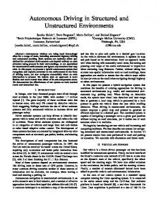
Fig. 2. Area of the Tuscany Archipelago. The red rectangle denotes the area of the Serious Game CTD survey. Red dots indicate the CTD station locations. (For interpretation of the references to color in this figure caption, the reader is referred to the web version of this paper.)

physical parameterisations. It provides initial and lateral boundary conditions for the SURF child components.

Fig. 1. Work-flow of SURF based on NEMO, SHYFEM and SWAN models.

parameter choices, the input datasets, and the spin-up time estimation. Forecast results and forecast validation are presented in Section 4, while the sensitivity study is discussed in Section 5. In Section 6 we present the conclusions.

2. SURF numerical components and methods 2.1. Numerical modelling platform SURF includes three basic components: (1) a structured grid hydrodynamic model based on the NEMO code (Madec, 2008); (2) an unstructured grid hydrodynamic model based on the SHYFEM code (Umgiesser et al., 2004; Bellafiore and Umgiesser, 2010); (3) a wave model based on the SWAN code (Booij et al., 1999). SURF is designed to be the “child” of a “parent” model which is normally at a lower horizontal and vertical resolution. The parent model could also have different numerical discretisation and

2.1.1. SURF standard structured grid component NEMO (Madec, 2008) is a primitive equation free-surface, finite differences 3-D ocean code suitable for modelling ocean circulation at regional and global scales. It solves the primitive equations (under the hydrostatic and Boussinesq approximations) along with a turbulence closure scheme and a nonlinear equation of state, which couples the two active tracers (temperature and salinity) to the fluid velocity. The 3-dimensional space domain is discretised by a structured Arakawa-C grid where the model state variables are horizontally/vertically staggered. This means that the freesurface, density, and active tracers are located at the center of the cell (T-grid), horizontal U and V velocities are located at the west/ east and south/north edges of the cell, respectively (U- and V-grid) and vertical velocity W is located at the bottom and top interfaces of cell (W-grid). In the vertical direction, the model can use a full or partial step z-coordinate, or s-coordinate, or a mixture of the two. We use stretched z-coordinate vertical layers, which are distributed along the water column, with appropriate thinning designed to better resolve the surface and intermediate layers. Partial cell parameterisation is used i.e. the bottom layer thickness varies as a function of position in order to fit the real bathymetry. Density is computed after the nonlinear equation of state of Jackett and Mcdougall (1995). Here we describe what is called the standard NEMO implementation which considers specific choices of physical parameterisations and boundary conditions. A horizontal biharmonic operator is used for the parameterisation of the lateral subgrid-scale mixing for both tracers and momentum. The horizontal eddy diffusivity and viscosity coefficients are parameterised as a function of the parent coarse resolution model. If a0 is the parent viscosity or diffusivity, the nested model equivalent coefficient is a ¼ a0 Δx4F =Δx4L , where ΔxF is the nested grid spacing and ΔxL is the large scale model grid resolution. The vertical eddy viscosity and diffusivity coefficients are computed following the Richardson-number dependent scheme of Pacanowski and Philander (1981). For cases where there might be unstable stratification, a higher value of 10 m2 =s is used for both viscosity and diffusivity coefficients.



3

Fig. 3. Left panel: bathymetry contour map of the Tuscan Archipelago as obtained from GEBCO datasets at 30 Arc seconds resolution. The red box highlights the subdomain region where we zoom in order to underline the structured and unstructured grid features (right panels). Right panels: horizontal grids for the subdomain region implemented by the structured (top panel) and unstructured (bottom panel) grid SURF models. The resolution of the structured grid corresponds to about 2 km, while the unstructured grid resolution ranges from 500 m near the coast up to 3 km in open sea. (For interpretation of the references to color in this figure caption, the reader is referred to the web version of this paper.)

The MUSCL (Monotonic Upstream Scheme for Conservation Laws) scheme is used for the tracer advection and the EEN (Energy and Enstrophy conservative) scheme is used for the momentum advection (Arakawa and Lamb, 1981; Barnier et al., 2006). No-slip conditions on closed lateral boundaries are applied and the bottom friction is modelled by a quadratic function with the additional coefficient of a turbulent kinetic energy due to tides and other unresolved processes (Lyard et al., 2006). We use a value of 2:5 103 m2 s 2 which is adopted in many other world ocean area (Killworth, 1992; Treguier, 1992). The surface wind, heat and water fluxes are computed through bulk formulas as described in Appendix A. Two different numerical algorithms to treat open boundary conditions are adopted depending on the prognostic simulated variables. For the barotropic velocities the Flather scheme (Oddo and Pinardi, 2008) is used, while for baroclinic velocities, active tracers and sea surface height we consider the flow relaxation scheme (Engerdahl, 1995). In our formulation we provide external data along straight open boundary lines and the relaxation area is equal to one internal grid point. As the parent coarse resolution MFS model provides only the total velocity field, the interpolated total velocity field into the child grid has been split into barotropic and baroclinic components. In order to preserve the total transport after the interpolation an integral constraint method is imposed (Pinardi et al., 2003). 2.1.2. SURF standard unstructured grid component SHYFEM (Umgiesser et al., 2004; Bellafiore and Umgiesser, 2010) is a finite element hydrodynamic code initially developed as a shallow water model and now fully 3D primitive equation model using the hydrostatic and the Boussinesq approximations. It

implements an unstructured Arakawa B horizontal grid (staggered finite elements). The domain is divided into triangular elements and the vertices of these elements are called nodes. SHYFEM computes scalars (temperature, salinity, water levels) on nodes and vectors (velocity) in the center of each element. It uses a semiimplicit time integration allowing maximum versatility in the definition of the horizontal resolution, which makes this code suitable for applications involving complicated geometry and bathymetry, such as those often encountered when modelling the coastal domain. As for the structured grid component of SURF, here we describe the standard set of physical parameterisations chosen for this exercise. The Pacanowski and Philander (1981) turbulence parameterisation is implemented in order to obtain vertical eddy viscosity and diffusivity coefficients. To compensate for unstable stratification, higher viscosity/diffusivity coefficients (10 m2 =s) are imposed. The horizontal advection scheme for the transport and diffusion equations is upwind, while the horizontal viscosity and diffusion scheme implements a Smagorinsky parameterisation (Smagorinsky, 1963, 1993). Air–sea physics and lateral boundary conditions are described in Appendix B. Lateral open boundary conditions are extracted from the parent coarse grid model distinguishing between scalar and vector quantities: the scalar parent fields (non-tidal sea surface height, temperature and salinity) are imposed at the boundary nodes, whereas the parent total velocities are specified only in the centre of mass of the triangular elements with two nodes attached to the boundaries. For more clarification and details about the lateral open boundary interpolation procedure refer to Federico et al. (2016). Flow relaxation scheme is imposed for temperature, salinity, SSH and total velocity only on the boundary lines.



4

Fig. 4. Vertical layer distribution of the simulations performed with the structured (top panel) and unstructured (bottom panel) grid components of SURF for the vertical sensibility study. The black line represents the reference experiment. We zoom on the first 100 m depth in order to provide informations concerning SURF vertical resolution in the upper layers where mixing is important, and on the thermocline resolution (30–50 m). The scale factor represents the distance Δz between each vertical layer and it is measured in meters.

The unstructured grid model component does not implement the integral constraint method introduced in Pinardi et al. (2003), it has been however checked that for short-time (7–10 days) simulations continuity equation violations are not relevant over the whole domain. 2.2. SURF wave model component The SWAN code (Booij et al., 1999) is a third generation spectral wave model designed to estimate wave conditions in small-scale, coastal regions with shallow water, (barrier) islands, tidal flats, local wind, and ambient currents. SWAN is based on the action balance equation which is solved with a full discrete twodimensional wave energy spectrum. An iterative technique is applied to allow propagation of waves in all directions over the domain in arbitrary conditions of wind, currents and bathymetry. The SWAN ocean code assembles all relevant processes of generation, dissipation and nonlinear wave-wave interactions in a numerical code that is efficient for small scale, high-resolution applications. The formulations of these processes in deep and intermediate-depth water in the present study are those that performed best in the validation and verification study of Booij

Fig. 5. Structured SURF-MFS (top panel) and unstructured SURF-MFS (central panel) total kinetic energy ratio for seven spin-up days computed on the entire Serious Game domain and considering only the coastal area (bottom panel). The coastal area is defined as the portion of basin that does not exceed a depth of 50 m. The target days fixed for the TKE computation are May 17, 2014 (blue lines) and May 21, 2014 (red lines). (For interpretation of the references to color in this figure caption, the reader is referred to the web version of this paper.)

et al. (1999) (see Table C1(c)). For wind input and whitecapping, we use the expressions of Komen et al. (1984), for quadruplet wave–wave interactions those of Hasselmann et al. (1985) and for bottom friction, those of Hasselmann et al. (1973). For triad wavewave interactions the expression of Eldeberky (1996) is used, and for depth-induced wave breaking a spectral version of the model of Battjes and Janssen (1978). In geographical space, the numerical



5

Fig. 6. RMSE (top panels) and BIAS (bottom panels) between the structured SURF solutions and CTD data (full dots) and between unstructured SURF solutions and CTD data (empty dots) for temperature (left panels) and salinity (right panels). RMSE and BIAS are calculated using the CTD data collected on May 17, 2014 (blue lines) and on May 21, 2014 (red lines). (For interpretation of the references to color in this figure caption, the reader is referred to the web version of this paper.)

scheme is a first-order upwind scheme. In spectral space (refraction and frequency shifting) a mixed upwind/central scheme is used for this study (Booij et al., 1999). 2.3. SURF work-flow SURF is working on a virtual machine environment where the three model components and several pre- and post-processing tools are connected to the numerical outputs and the required inputs fields. Also a non-virtual machine is suitable to run SURF since the user access to the source code and executable. The preand post-processing tools are specifically developed and optimised for SURF in order to reduce the latency of the computation and to have efficient memory usage. The three main hydrodynamic and wave model components are written in fortran and the pre- and post-processing tools used are developed in NCL, NCO and python programming languages. In the following, we briefly describe the work-flow of the SURF numerical platform as shown in Fig. 1. The first step consists in the choice of the ocean model simulation parameters for NEMO or SHYFEM, and SWAN. The parameters are listed in Table C1((a)–(c)) for each model component. The second step concerns the access to the following input datasets: (1) bathymetry; (2) coastline; (3) parent model U; V; T; S ; η fields and (4) the atmospheric forcing dataset.

After the model configuration and the input data acquisition, the generation of the numerical grid is performed. For a finite element simulation, an unstructured grid is required and its generation is not automatic yet. In this case a few interactive steps are required. The next automatic step is the data reformat, which generates the forcing, boundary and initial condition dataset on the child grid that are needed to run the model. Input dataset fields are interpolated into the child grid, using Kara et al. (2007) and De Dominicis et al. (2014). As it is explained in these references, we adopt the so-called sea-over-land (SOL) procedure that provides us with the field values on the areas near the coastline where the parent model solutions are not defined. The SOL procedure extrapolates iteratively the ocean quantities on the land gridpoints, so that it is possible to interpolate these quantities on the child grid. This applies also to atmospheric fields in order to avoid land contaminations near the land-sea boundaries. Horizontally bilinear interpolation method is adopted for the structured grid component, while for the unstructured grid component the Cressman's interpolation technique (Cressman, 1959) is used. In the vertical direction, a liner interpolation is performed for both model components. Finally, the SURF platform proceeds with numerical integration and produces the final outputs. Visualisation procedures can be



6

Fig. 7. Averaged daily temperature on May 17, 2014 of the parent MFS model (left panels), the structured (central panels, top rows) and unstructured (central panels, bottom rows) grid SURF, the difference between SURF and MFS models (right panels).

activated in order to display the resulting field profiles on the SURF UI. For the time being, coupling between the wave model and the hydrodynamic is univocal. Once current fields have been obtained by SURF, wave predictions can be produced starting from these fields. Waves themselves do not affect or produce ocean currents.

3. Case study: the Tuscan Archipelago The relocatable nested-grid modelling system SURF is implemented in the Tuscan Archipelago, the area between the Ligurian Sea and the Tyrrhenian Sea, as highlighted in Fig. 2. The Tuscany Archipelago test case is chosen because two CTD surveys were carried out to validate the forecasting skill of the structured and unstructured model components of SURF. Two synoptic cruises were organised in the days 17th and 21st of May 2014 with the contemporary acquisition of physical and bio-chemical data from two different vessels. These cruises were part of the activities of the Serious Game exercise organised in the eastern Ligurian Sea in the framework of the MEDESS-4MS project, co-funded by the Med Programme. The hydrological grid had a horizontal resolution of 3 nm with CTD 45 stations also inside an oil slick located in an area of about 70 km 2 north of the Elba island (Fig. 2, red rectangle). This area is characterised by a high level risk for oil spills but no previous in-depth environmental studies are present. Aim of the Serious Game exercise was to acquire data to characterise the area for the first time and validate a circulation numerical model and an oil spill numerical model realised in the framework of the

MEDESS-4MS project and part of its oil-spill management online system. Physical and bio-chemical data were collected using a CTD Seabird SBE19 equipped with sensors of pressure, temperature, conductivity, dissolved oxygen, turbidity, Chl α and CDOM fluorescence. In situ data collection activities were performed on board of the vessels made available by the Italian Coast Guard and used as Ships of Opportunity. The two surveys collected hydrological data each in about 24 h, thus realising a synoptic estimate of the thermocline properties of the area. CTD data collection has a grid spacing of approximately 5– 6 km, therefore experimental data are able to resolve the Rossby radius, which corresponds to about 10 km in the Mediterranean sea. This is a quite shallow area between two sub-basins of the western Mediterranean, the Ligurian sea at north and the Tyrrhenian sea at south. Wind and bathymetry influence the hydrodynamic characteristics of the area with mainly northward MAW at the surface and a clear seasonal thermocline that separates two different dynamics at 40–50 m depth. There are an upper layer with cyclonic and anti-cyclonic gyres 20–30 km in diameter, also described by Robinson et al. (2002a), mixing the surface waters mainly driven by winds and a deeper layer with a lower dynamics driven by the bottom morphology. 3.1. The model set-up Table C2 summarises the values chosen for the reference experiment, concerning the structured grid (left column) and unstructured grid (right column) components of SURF.



7

Fig. 8. Averaged daily temperature on May 21, 2014 of the parent MFS model (left panels), the structured (central panels, top rows) and unstructured (central panels, bottom rows) grid SURF, the difference between SURF and MFS models (right panels).

3.1.1. Structured grid model The left panel in Fig. 3 shows the horizontal domain of the structured grid component of SURF. We set the grid spacing ratio to 3, meaning that the child domain has a grid spacing that is one third the size of the of the parent domain. Parent and child models are linked through their lateral interface, where the results of the coarser grid model are used to specify the boundary conditions for the finer grid model. The nested domain can be placed anywhere within the parent domain and the location of grid points of the parent model does not necessarily have to coincide with the grid points of the child model. However, in order to reduce the errors due to interpolation procedures, the coarse and fine grids have been exactly overlapped: each point of the coarse grid lies exactly on the fine grid. The model domain is a 200 km longitude by 257 km latitude area, extending from 9:381E to 11:851E and from 42:061N to 44:37 1N , it consists of 120 112 grid points in the horizontal plane with a resolution of 1=481 (about 2 km). A portion of the structured horizontal grid is shown on the right top panel of Fig. 3. On the vertical axis the levels of the parent and child domains are the same and consist of 53 z-levels with a stretching factor of hcr ¼ 30 and a model level with maximum stretching of hth ¼ 101:8. They are smoothly distributed from 1.47 m to the maximum depth of the selected nested domain (1529 m) and have level thickness that increases with depth from approximately 3–120 m. The vertical location of W- and T-levels is defined from the reference coordinate transformation zðkÞ given by zðkÞ ¼ hsur h0 k h1 log ½coshðÞk hth Þhcr Þ

ð1Þ

where the coefficients hsur, h0, h1, hth and hcr are free parameters to

be specified. hcr represents the stretching factor of the grid and hth is approximately the model level at which maximum stretching occurs (see A.2 for more details). The vertical layer distribution considered in the reference experiment is shown in Fig. 4 (top panel, black line). 3.1.2. Unstructured grid model The unstructured SURF model is implemented in the domain shown in Fig. 3, left panel. The horizontal mesh consists of 31 408 nodes and 61 190 elements, with a resolution tuned in order to better resolve the coastlines, from 500 m near the coast up to 3 km in open sea. The high resolved region extends up to 1 km from the coastline where the grid starts to increase its resolution. The maximum size of the unstructured grid elements corresponding to 3 km is reached after a distance of 50 km from the coastlines. The unstructured horizontal mesh is shown on the right bottom panel of Fig. 3. The vertical grid consists of 38 z-levels that are smoothly distributed along the water column: the spacing between the vertical layers should be as much homogeneous as possible in order to minimise the errors coming from vertical partial derivatives discretisation. Moreover, it presents an appropriate thinning designed to better resolve the surface and intermediate layers. The vertical distribution of these layers is shown in Fig. 4 (bottom panel, black line). 3.2. Input datasets The bathymetry is obtained from the General Bathymetric Chart of the Oceans (GEBCO) datasets by linear interpolation of the



8

Fig. 9. Averaged daily current fields on May 17, 2014 of the parent MFS model (left panels), the structured (central panels, top rows) and unstructured (central panels, bottom rows) grid SURF, the difference between SURF and MFS models (right panels).

depth data into the SURF model grid (see Fig. 3, right panel). This dataset contains the ocean depths (in meters) at 30 arcsec resolution defined on a regular horizontal grid and covering the whole globe. The initial and lateral boundary conditions for SURF are extracted from the operational MFS daily mean data available on the Copernicus Marine Environment Monitoring Service (CMEMS) portal, from which we download temperature, salinity, sea surface height (η) and total velocity ðU; VÞ fields. The MFS model has an horizontal resolution of 1=161 and 72 unevenly distributed layers in the vertical direction. The atmospheric fields containing wind velocity, temperature, humidity and surface pressure are extracted from the European Center for Medium-Range Weather Forecasts (ECMWF) operational analyses, which have a 6 h frequency and spatial resolution of 0:1251. The instantaneous precipitation values are computed from the ECMWF operational forecast accumulated precipitations at a frequency of 3 h and 0:251 spatial resolution.

3.3. Model spin-up time The spin-up time is defined as the time necessary by the child ocean model to reach a steady state value for the volume average kinetic energy starting from initial and lateral boundary conditions interpolated from the parent model (Simoncelli et al., 2011). We analyse the spin-up issue by fixing a target IC at day (J) and running several experiments starting from J-1, J-2, … days before the target day. The total kinetic energy (TKE) of the SURF velocity field is computed for each experiment considering the following

expression: Z 1 ðU 2 þ V 2 Þ dx dy dz TKE ¼ Vol Vol 2

ð2Þ

at the target day J. The spin-up experiment is repeated for the target day May 17, 2014 and May 21, 2014. The total kinetic energy (TKE) of the SURF model components is compared to the kinetic energy of MFS computed on the same region, obtaining the behaviour presented in Fig. 5. The structured grid model result for this comparison is shown on the top panel, while the middle panel presents the unstructured grid model TKE. This ratio is computed on two different target days, May 17, 2014 and May 21, 2014, for different spin-up day simulations. For the structured model spin-up time, it clear from the top panel of Fig. 5 that the first three days TKE grows twice as much as the following days. Following this criteria, we adopt for the structured grid model a spin-up period of four days. For the unstructured grid model (Fig. 5, middle and bottom panels) the “plateau” is better defined and we consider the spin-up time to be four days as well. The comparison between the top and middle panels of Fig. 5 also highlights that the TKE contribution from the unstructured grid model is higher than the one resulting from the structured grid model. This is a consequence of the resolution increase, mostly along the coastlines, of the unstructured grid model of SURF, as confirmed by the computation of the costal TKE, which is shown in the bottom panel in Fig. 5. For this computation, we consider the portion of the simulated basin that does not exceed a depth of 50 m. This result illustrates how the major component of SURF TKE originates from the highly resolved coastal dynamics. The TKE ratio curve is very different for different target days and different models. The unstructured SURF model for day 21



9

Fig. 10. Averaged daily current fields on May 17, 2014 of the parent MFS model (left panels), the structured (central panels, top rows) and unstructured (central panels, bottom rows) grid SURF, the difference between SURF and MFS models (right panels).

shows a decrease in the TKE ratio for 3–5 days of spin up. Nevertheless the ratio reaches a plateau, but in one case the energy increases to a high limit value while in the other the child TKE decreases thus increasing the spin-up time. In order to test and quantify the accuracy of the assumption that four days is sufficient for the solution to adapt to the higher resolution grids adopted by SURF, we evaluate the root mean square error (RMSE) and BIAS between the quantities simulated by each model ψm and the observed quantities ψo, defined by: vffiffiffiffiffiffiffiffiffiffiffiffiffiffiffiffiffiffiffiffiffiffiffiffiffiffiffiffiffiffiffiffiffiffiffiffi u N u1 X RMSE ¼ t ðψ m ψ o Þ2 ð3Þ N i BIAS ¼

N 1X ðψ m ψ o Þ N i

ð4Þ

where N is the total number CTD data at our disposal and ψ stands for either temperature or salinity. We interpolate both SURF and MFS results over the CTD data depths, then we compute the RMSE between data and simulations within 5 m intervals along each CTD cast. CTD measurements reach different sea depths, but only 10 CTD stations concern depths deeper than 100 m, therefore we show the RMSE values only up to this maximum depth. Below 100 m we do not consider the result statistically significant. The result of this computation is shown in Fig. 6. As explained above, we preform several simulations for different spin up days, and we compute RMSE and BIAS values on two target days corresponding to the CTD data collection days, May 17, 2014 (blue lines) and May 21, 2014 (red lines). Fig. 6 shows the RMSE (top panels) and the BIAS (bottom panels) obtained considering the

structured SURF solutions (full dots) and the unstructured SURF solutions (empty triangles) for temperature (left panels) and salinity profiles (right panels). The behaviours of the RMSE and the BIAS shown in Fig. 6 confirm that the more spin-up days we consider the smaller difference between simulated solutions and CTD data we get. At the same time, it is well known that boundary condition errors influence the predicted fields inside the simulated domain and propagate at a finite speed. The best compromise is to get relatively short spin-up time in order to achieve longer forecast.

4. Forecast validation As discussed in Section 3.3, we consider four days as a sufficient spin-up time for SURF. We then compare daily mean temperature and current fields for May 17, 2014 and for May 21, 2014, after 4 days of forecast. Figs. 7 and 9 display temperature and current fields respectively, averaged from 12:00 UTC of May 16 to 12:00 UTC of May 17 as obtained with the structured (middle panels, top row) and unstructured (middle panels, bottom row) grid SURF components and MFS model (left panels). The differences between SURF and MFS models are shown in the panels on the right for the structured (top row) and unstructured (bottom row) grid components. The first general consideration is that the flow field generated by both SURF high-resolution components is more intense than the parent model flow. This is confirmed by the TKE computation performed in Section 3.3, where the SURF/MFS TKE ratio on May 17 2014 after 4 spin-up days for the structured and the unstructured grid components is 1.18 and 1.61 respectively. More in


10


Fig. 11. RMSE between the structured SURF solutions and CTD data (red dots) and between MFS results and CTD data (blue dots) for temperature (left panels) and salinity (right panels). The CTD data considered for this comparison were collected on May 17, 2014 (top panels) and on May 21, 2014 (bottom panels). (For interpretation of the references to color in this figure caption, the reader is referred to the web version of this paper.)

details, the SURF models reveal the circulation near the coasts and around the Elba island. The Eastern Corsica current (Pinardi et al., 2015) which flows northward between Corsica and Capraia (Figs. 7 and 9) turns southward after Capraia forming a free flowing jet north-east of Capraia which merges with an anticyclonic eddy to the south. The flow field in the area of the CTD survey is weak while all around the flow is characterised by jets and boundary currents. Along the Tuscany coastlines the currents are dominantly southward and an intense westward boundary current is present north of the Elba island. A large current develops in the SURF models between the coastlines and the Elba island, stronger but noisier in the structured than the unstructured grid SURF model components. Figs. 8 and 10 present the evolution on May 21, 2014 after four days forecast. As already discussed for May 17, 2014, even on May 21, 2014 the high-resolution flow fields are more intense than the coarse-resolution model flow, as confirmed by values of 1.1 for the structured grid TKE ratio and 1.4 for the unstructured grid case. The averaged current increases with respect to May 17 and spreads east of Capraia deleting the free flowing jet and the anti-cyclonic

eddy which where visible in the initial conditions. In the CTD survey region, the flow field increases as well compared with May 17, and an intense north-eastward jet forms east of Capraia. The currents along the Tuscany coastline turn northward. Another consequence of the Eastern Corsica current intensification is that the boundary current north of the Elba island turns eastward. The general flow field increase described above is related with an increase in temperature with respect to May 17, 2014, as shown in Figs. 7 and 8. This temperature increase is stronger in the unstructured than the structured grid SURF model components and this is related with higher current flow field and TKE ratio values on May 21, 2014 reported above. In order to test and quantify the real improvement obtained by the higher resolution SURF model compared to the parent coarse resolution MFS model, we evaluate the RMSE and the BIAS between the quantities simulated by each model and the observed quantities, as obtained using Eqs. (3) and (4) respectively. The RMSE resulting from the comparison between SURF results at different depths and CTD data is shown in Fig. 11 (structured grid



11

Fig. 12. BIAS between the structured SURF solutions and CTD data (red dots) and between MFS results and CTD data (blue dots) for temperature (left panels) and salinity (right panels). The CTD data considered for this comparison were collected on May 17, 2014 (top panels) and on May 21, 2014 (bottom panels). (For interpretation of the references to color in this figure caption, the reader is referred to the web version of this paper.)

model) and 13 (unstructured grid model) for May 17 (top) and May 21 (bottom panels). Left panels display the results obtained by comparing model outputs with CTD temperature measurements, while the salinity comparison is shown in the panels on the right. Red dots denote RMSE values obtained by SURF forecast results, while blue dots are MFS RMSE values. Equivalently, Figs. 12 and 14 present the BIAS results for the structured and unstructured grid component simulations respectively. The improvement in both the structured and unstructured SURF model compared to the MFS model is highlighted by the predominance of the green regions over the red regions. In order to better quantify this improvement, we compute the water column averaged RMSE and BIAS values, which are listed in Table C3. It is clear from these values that SURF platform models are improving the forecast quality with respect to MFS model of 10–15%, as resulting from both RMSE and BIAS profiles computation. Even without assimilating data, the additional resolution offered by SURF model components is capable to improve the quality of the predictions.

4.1. Wave model results As a demonstration experiment, we show here the one way coupling of SWAN with the structured and unstructured SURF model components. SWAN run on a structured mesh and use same domain size and grid resolution adopted for the ocean circulation model (Fig. 3) with a 1=481 (about 2 km) resolution for the structured grid circulation model component and a 1=1001 (about 1 km) resolution for the unstructured grid circulation model component. In the latter case the resulting current fields defined on a unstructured mesh are interpolated on a regular grid and the resolution of 1=1001 is chosen in order not to loose the informations concerning the highly resolved costal area. The SWAN integration time step is 1800 s. The wave frequencies range from 0.04 to 1.5 Hz and are discretised into 35 bins on a logarithmic scale (Δσ =σ 0:1). The wave directions cover the full 3601 and are discretised into 36 sectors, each sector representing 101. SWAN is driven by wind speeds and sea surface currents. Wind velocity fields are obtained by linear interpolation of the ECMWF


12


Fig. 13. RMSE between the unstructured SURF solutions and CTD data (red dots) and between MFS results and CTD data (blue dots) for temperature (left panels) and salinity (right panels). The CTD data considered for this comparison were collected on May 17, 2014 (top panels) and on May 21, 2014 (bottom panels). (For interpretation of the references to color in this figure caption, the reader is referred to the web version of this paper.)

atmospheric analyses (0.25 and 6 h) on the SURF high resolution grid. Two different sea surface current fields can be passed to SWAN: (1) the parent model (MFS) current interpolated on the SURF high resolution grid and (2) the high resolution current obtained by the structured and unstructured hydrodynamic model components of SURF. The SWAN simulation starts on May 17, 2014 at 00:00 and run until May 21, 2014 at 24:00. Fig. 15 shows the significant wave height and wave direction on May 19, 2014 at 18:00:00 as computed by SURF-SWAN. The wave model is forced by the sea surface current obtained by the MFS model (left panels), the structured (middle panels, top row) and unstructured (middle panels, bottom row) grid SURF components. The difference in magnitude between the significant wave height with MFS current (interpolated onto the nested grid) and SURF current are shown in the right panels for the structured (top row) and unstructured (bottom row) grid components. The significant wave height produced by SWAN with MFS and SURF currents are similar with values between 0 and 1.2 m and the resulting wave directions are consistent. This result is a direct

consequence of the major influence of the wind velocity field which is common to MFS and SURF components. On the other hand, we note a significant wave height increase for the wave simulation forced by the unstructured grid current field (bottom panels of Fig. 15) and this can be related with a stronger sea surface current obtained by this model simulation. The resulting wave direction is instead very consistent between the different SURF coupling.

5. Sensitivity study The final step in our analysis examines the robustness of our results according to the reference experiments. We thus perform the sensitivity study summarised in Table C4. Our aim is to understand how the improvements obtained by the higher resolution model SURF responded when we modify the vertical grid resolution or the vertical turbulence scheme.



13

Fig. 14. BIAS between the unstructured SURF solutions and CTD data (red dots) and between MFS results and CTD data (blue dots) for temperature (left panels) and salinity (right panels). The CTD data considered for this comparison were collected on May 17, 2014 (top panels) and on May 21, 2014 (bottom panels). (For interpretation of the references to color in this figure caption, the reader is referred to the web version of this paper.)

In order to understand the effects of these modifications, we compute for each experiment the following quantity: SSexp ¼ 1

RMSE exp 100% RMSEMFS

ð5Þ

This expression identifies the so-called RMSE skill score (SS) and can be interpreted as the improvement in percentage of a forecast with respect to a reference. For a perfect forecast the SS will be 100%, while 0% indicates no improvement over the reference MFS analysis forecast. A negative value of SS highlights a region where the SURF experiment gives worse predictions compared to MFS outputs. 5.1. Effect of vertical resolution The first aspect that we investigate is the effect of the different distribution of vertical levels. One important issue is at what depths more layers should be distributed in numerical ocean models. However, this depends on which phenomena should be simulated the most realistically, which score should be improved the most, and to what extent each physical parameterisation

(mixing layer and bottom boundary layer) should exploit vertical high resolution level distribution. A stretched vertical coordinate is used in both the structured and unstructured SURF model so that finer spacing is assigned to the upper ocean while coarser vertical spacing is applied at lower levels. The finer vertical grid is used to accommodate the rapid change in ocean variables in the top ocean layer and to resolve the small-scale features near the surface, while the coarser grid at lower levels is used to reduce computational cost. Concerning the structured grid model, the vertical location of the W- and T-levels is determined by the number of levels nz, the bathymetry and the analytical coordinate transformation z(k). The standard transformation for a z-coordinate in NEMO (Eq. (1) in Appendix A.2) includes five free parameters hsur, h0, h1, hth and hcr and defines a nearly uniform vertical location of levels at the ocean top and bottom with a smooth hyperbolic tangent transition in between. To illustrate the effects of varying the vertical level distribution on the accuracy of our simulations, a small number of experiments are performed (Table C4(a)). Specifically, we consider three different vertical level distributions, obtained by varying the values of the stretching parameter hcr (LEV-S1), the parameter hth


14


Fig. 15. Significant wave height contours (m) and wave direction on May 19 2014 18:00 as computed by SWAN. The wave model is forced by the sea surface currents obtained by the MFS model interpolated on the structured (left top panel) and unstructured (left bottom panel) grids, the structured (middle panel, top row) and unstructured (middle panel, bottom row) grid SURF components. The difference between SURF and MFS models are shown in the right panels.

(LEV-S2) and the number of levels nz (LEV-S3) as shown in Fig. 4 top panel (blue, green and red lines respectively). For each experiment considered in this sensitivity analysis, we fix the values (reference model values) for all the other model parameters. The top panels in Fig. 16 show the effect of different vertical distributions in the computation of the RMSE skill score computed for the reference experiment REF-S (black line), LEV-S1 (blue line), LEV-S2 (green line) and LEV-S3 (red line). Increasing the vertical stretching (smaller parameter hcr value) leads to a finer vertical grid spacing at the top layer of the ocean and coarser vertical spacing at the bottom boundary layer. This leads to an higher skill score for both temperature and salinity within the upper ocean surface layer. A decrease in the parameter hth value (LEV-S2) results in an upward shift of the model vertical level at which maximum stretching occurs and so leads to a lower vertical resolution in the top ocean layer. This leads to a lower skill score for both temperature and salinity within the upper ocean surface layer. Finally, doubling the number of levels causes a higher vertical resolution in the top ocean layer which is maintained between 3 and 4 m. This improves in performance for both temperature and salinity within the upper ocean surface layer. Concerning the unstructured grid component of SURF, we double the vertical resolution used in the reference experiment. LEV-U1 adopts a total of 74 vertical layers distributed as shown in the bottom panel of Fig. 4 (red line). We compare the forecast obtained by the reference experiment and by LEV-U1 for May 17, 2014 and compute the RMSE between these experiment outputs

and the CTD data collected on this day. The top panels of Fig. 17 show the effect of the increase of vertical discretisation in the RMSE skill score computed for the reference experiment (black line) and for LEV-U1 (red line). Doubling the vertical layer distribution does not induce any visible improvement in the subsequent model forecast, both for temperature and salinity profiles in the first 60 m. The skill score related to the finer vertical discretisation increases only within the lower ocean layers. 5.2. Effect of vertical mixing In this section, we assess the effectiveness of different vertical turbulent schemes available in NEMO and SHYFEM. Vertical mixing plays an essential role in ocean dynamics and must therefore be correctly estimated. It creates the mixed layer, the homogeneous ocean layer that interacts directly with the atmosphere, which can then be modelled as the mixed layer depth (MLD). The MLD plays a very important role in the energetic exchanges between the ocean and the atmosphere and can have very high spatial and temporal variations. The analysis concerning the structured grid component of the SURF platform compares two different vertical mixing parameterisations: as already specified, the reference experiment REFS adopts a PP parameterisation (Pacanowski and Philander, 1981), while TURB-S1 chooses the Generic Length Scale (GLS) parameterised as a k–ϵ closure model (Rodi, 1987). The results of this comparison for May 17 are shown in the bottom panels of Fig. 16. Within the upper layer of the ocean



15

Fig. 16. RMSE skill score for the structured grid component of the SURF platform comparing four different vertical stratifications (top panels) and two different vertical turbulence schemes (bottom panels). Temperature (left panels) and salinity (right panels). Skill score is computed considering CTD vertical profiles collected on May 17, 2014. The black line represents the SURFS reference experiment.

(z o 30 m), the skill score for both temperature and salinity is slightly higher using the PP parameterisation with respect to GLS parameterisation. Deeper than 30 m both temperature an salinity seems not to be affected by vertical mixing scheme variations. The analysis concerning the unstructured grid component of SURF platform compares three different vertical mixing parameterisations: as already specified, the reference experiment REF-U adopts a PP parameterisation (Pacanowski and Philander, 1981); TURB-U1 chooses the k-ϵ module of General Ocean Turbulence Model (GOTM) described in Burchard and Petersen (1999); TURB-U2 implements a variation of the classical PP scheme presented in Lermusiaux (2001). This modification mimics the wind effect on the surface layer mixing by imposing constant high values of vertical viscosity (ν ¼ 0:01 m2 =s) and diffusivity (k ¼ 0:0001 m2 =s) for a fixed surface layer. The depth of this surface layer hmodPP is controlled by the parameter ϵk, which fixes the fraction of the Ekman layer above which “wind mixing” applies (hmodPP ¼ ϵk hEkman ). Below this surface layer the classical PP scheme applies.

The results of this comparison for May 17 are shown in the bottom panels of Fig. 17. The major differences concern temperature profiles, which show that the modification of the PP scheme (TURB-U2) better captures the surface temperature than the other two mixing parameterisations. Salinity seems not to be affected by vertical mixing scheme variations, at least for shorttime simulations.

6. Summary and conclusions In this paper we have described a new relocatable ocean model platform used to increase resolution or downscale the large scale ocean model fields from operational ocean forecasting systems. The concept is to use initial and lateral boundary conditions from these large scale models and increase resolution and processes only when and where they are needed, especially in the coastal areas and in the vertical direction. The platform contains both structured and unstructured grid models and a wind wave model coupled one way to the hydrodynamics models.


16


Fig. 17. RMSE skill score for the unstructured grid component of the SURF platform comparing two different vertical stratifications (top panels) and three different vertical turbulence schemes (bottom panels). Temperature (left panels) and salinity (right panels). Skill score is computed considering CTD vertical profiles collected on May 17, 2014. The black line represents the SURFU reference experiment.

The SURF components are described in details and the conditions for initialization and lateral boundary condition imposition elucidated. It is found that only few days are required for both the structured and unstructured grid models to dynamically adjust the coarse initial conditions. Furthermore, SURF models are capable to adjust without shocks the coarse interpolated/extrapolated initial conditions. The SURF downscaling is compared with observed temperature and salinity profiles collected during the Serious Game CTD survey in the Tuscan archipelago. It is shown how the nested models, structured SURFS and unstructured SURFU, provide an improved ocean forecast with respect to the parent MFS model. The better resolution of open ocean mesoscale dynamics and the better representation of the coastal geometry and bathymetry allows to decrease RMSE and BIAS of SURF forecasts with respect to MFS when compared with observations. The SURFS and SURFU currents are interfaced with the wind wave model which shows sensitivity to the currents used, especially the unstructured grid model currents.

Finally a sensitivity case study is performed, showing the impacts of different vertical level distributions and vertical mixing parameterizations on the quality of the forecast. It is found that doubling the levels does not change appreciably the RMSE and BIAS scores for the short term forecasts probably due to the fact that the vertical dynamics is inhibited during the May months. In conclusion, the SURF platform has been shown to be a useful tool for dynamical downscaling. This study allows us to confidently initialize our model in order to produce short-time forecasts that will improve predictions for other application models, such as drifting objects trajectories or oil spill transport and transformation. Future developments should consider the inclusion of coupled wind wave-current dynamics in the hydrodynamics models, the inclusion of tides in the lateral boundary conditions, and the usage of SURF as an ensemble forecasting tool to quantify uncertainties in forecasts in different world ocean coastal areas.



coefficients, respectively e AlT;S , AvT;S are the horizontal and vertical eddy diffusivity coefficients, respectively.

Acknowledgement This work has been founded by TESSA and ATLANTOS Projects. We thank Alberto Ribotti (IAMC CNR, Oristano, Italy) for providing CTD data.

Appendix A. Description of the finite difference code NEMO A.1. Governing Equations NEMO (Nucleus for European Modelling of the Ocean (Madec, 2008), www.nemo-ocean.eu is a primitive equation free-surface, finite differences 3-D ocean model developed at Institut Pierre Simon Laplace (IPSL-CM), suitable for modelling ocean circulation at regional and global scales. It prognostically solves (under the hydrostatic and Boussinesq approximations) primitive equations, along with a turbulence closure (selected from various options) and a nonlinear equation of state which couples the two active tracers (temperature and salinity) with the fluid velocity. The vector invariant form of the primitive equations in the (i,j,k) vector system provides the following six equations: ∂Uh 1 1 ¼ ω U ∇ðU2 Þ f k Uh ∇h P þ DU 2 ∂t ρ0

ðA:1Þ

∂p ¼ ρg ∂z

ðA:2Þ

∇U¼0

ðA:3Þ

∂θ ¼ ∇ θU þ DT ∂t

ðA:4Þ

∂S ¼ ∇ ðSUÞ þ DS ∂t

ðA:5Þ

ρ ¼ ρðθ; S; pÞ

ðA:6Þ

where U ¼ ðu; v; wÞ is the three-dimensional velocity field, Uh is the horizontal velocity field, ∇ is the generalised derivative vector operator in (i,j,k) directions, t the time, z the vertical coordinate, ω ¼ ∇ U is the vorticity field, θ, S, p are, respectively, the potential temperature, salinity and pressure, f ¼ 2Ω k is the Coriolis parameter, Ω is the Earth angular velocity, g the gravitational acceleration, ρ0 a reference density, ρ the in situ density given by the modified UNESCO equation of state formula by Jackett and Mcdougall (1995). This formulation allows the computation of the in situ ocean density ρ directly as a function of potential temperature θ (instead of the in situ one T), the salinity S and the pressure p

ρ ¼ ρðθ; S; pÞ ¼

ρðθ; S; 0Þ 1 p=Kðθ; S; pÞ

ðA:7Þ

where ρðθ; S; 0Þ ¼ ρðT; S; 0Þ (since θ ¼ T at p¼ 0) is a 15-term polynomial containing various products of powers of S and θ and Kðθ; S; pÞ is a 26-term polynomial with powers of θ, S e p. DU , DT e DS are the parameterizations of sub-grid scale physics for momentum, temperature and salinity, including surface forcing terms. They are divided into a lateral part DlU , DlT and DlS and a vertical part DvU , DvT and DvS: ∂ ∂U Avm ðA:8Þ DU ¼ DlU þ DvU ¼ Alm ∇4 U þ ∂z ∂z DT ¼ DlT þ DvT ¼ AlT ∇4 θ þ DS ¼ DlS þ DvS ¼ AlS ∇4 S þ

17

∂ ∂θ AvT ∂z ∂z

∂ ∂S AvS ∂z ∂z

ðA:9Þ ðA:10Þ

where Alm, Avm are the horizontal and vertical eddy viscosity

A.2. Spatial discretization The NEMO governing equations are spatially discretised in finite differences on a staggered Arakawa C-grid (Arakawa and Lamb, 1977), i.e. with sea level height (η), density (ρ) and active tracers (T,S) located at the center of grid cells and velocities (u, v and w) located at the center of the grid faces (west/east, south/ north, up/down faces of the cells, respectively). In the horizontal direction, the model uses a orthogonal curvilinear coordinate system which allows cartesian, polar and spherical coordinates applications. The transformation of these coordinates to the model grid is specified in metric terms. In particular, the SURF model adopts a regular spatially latitude/longitude grid in a spherical coordinate system. The horizontal grid must be defined by setting the number of points nλ and nφ in the zonal and meridional directions respectively, the grid sizes Δλ and Δφ (expressed in degrees) and the reference longitude and latitude coordinate ðλ; φÞ11 , which corresponds to the lower left corner of the T-grid. In the vertical direction, the model uses a full or partial step z coordinate, or s coordinate, or a mixture of the two. In particular, the SURF model adopts a stretched z coordinate vertical levels which are smoothly distributed along the water column, with appropriate thinning designed to better resolve the surface and intermediate layers. The vertical location of W- and T-levels is defined in Eq. (1). This expression allows us to define a nearly uniform vertical location of levels at the ocean top and bottom with a smooth hyperbolic tangent transition in between. Partial cell parameterisation is used i.e. the thickness of the bottom layer is allowed to vary as a function of geographical location ðλ; φÞi;j to allow a better representation of the bathymetry. With partial steps, the deepest layer nz 1 of the model is allowed to have either a smaller or larger thickness than e3t ðnz Þ: the maximum thickness Δzbmax allowed is 2 e3t ðnz 1Þ, the minimum thickness allowed is given by

Δzbmin ¼ MINðe3zps_min; e3zps_rat n e3t Þ

ðA:11Þ

where e3zps_min and e3zps_rat are free parameters to be specified and represent, respectively, the minimum thickness (in meters) and the fraction of the default thickness e3t ðnz Þ. The advection scheme for active tracers is a MUSCL (Monotonic Upstream Scheme for Conservation Laws, (Van Leer, 1979), as implemented by Lévy et al. (2001)) scheme. This is a second order, TVD (total variation diminishing) spatial discretisation scheme that provide highly accurate numerical solutions for our system, even in cases where the solutions exhibit discontinuities or large gradients. The momentum advection scheme used is the EEN (Energy and Enstrophy conservative) scheme. In this scheme the discrete formulation of the vorticity term provides a conservation of both horizontal kinetic energy and potential enstrophy in the limit of horizontally non-divergent flow (Arakawa and Lamb, 1981). A.2.1. Time-stepping The model time stepping environment used in NEMO is a three level scheme in which the tendency terms of the equations are evaluated either centred in time, or forward, or backward depending on the nature of the term. The time central difference scheme, known as the leapfrog method (Mesinger and Arakawa, 1976) associated with a Robert–Asselin time filter (Asselin, 1972) is used for momentum and tracer advection, pressure gradient, and Coriolis terms. For the horizontal and vertical diffusion terms, a forward and backward scheme, respectively, are used. Explicit, split-explicit and filtered free surface formulations are implemented for solving the prognostic equations for the active



18

tracers and the momentum. The SURF model adopts the splitexplicit free surface formulation, also called the time-splitting formulation, follows the one proposed by Griffies (2004) which splits the fast barotropic part and the slow baroclinic part of the dynamics. According to this formulation, the depth varying prognostic variables (baroclinic velocities and tracers) that evolve more slowly are solved with a larger time step Δt (depending on the horizontal resolution) while the barotropic part of the dynamical equations is integrated explicitly with a short time step Δt e (the external mode or barotropic time step) which is provided through the nn_baro name-list parameter as: Δt e ¼ Δt=nn_baro. A.3. Numerical boundary condition algorithms At the surface, the momentum, salinity, and heat fluxes are prescribed by ∂U τ ¼ ðA:12Þ Avm h ∂z z ¼ η ρ0 AvS

∂S ¼ ðE PÞS ∂z z ¼ η

∂θ AvT ∂z

z¼η

¼

Q ns

ðA:13Þ

where τ is the wind stress, E and P are the evaporation and the precipitation budget, C p ¼ 4000ðJ=Kg KÞ is the ocean specific heat and Qns is the non-solar heat flux, the no-penetrative part of the net surface heat flux Q (positive when received by the ocean). The net surface heat flux Q is split into four terms: Q ¼ Q sr þ Q lw þ Q s þ Q e |fflfflfflfflfflfflfflfflfflfflfflfflffl{zfflfflfflfflfflfflfflfflfflfflfflfflffl}

ðA:15Þ

Q ns

where Qsr is the solar heat flux, Qlw is the long-wave contribution to the net radiation received at the sea surface, Qs is the sensible heat flux and Qe is the latent heat flux. To evaluate the surface heat balance, the atmospheric fluxes are computed through bulk formulas, as implemented in MFS (Pettenuzzo et al., 2010). At the bottom, the normal component of velocity is zero, no flux of heat and salt are applied and the friction is modelled by a quadratic function. These conditions are expressed, respectively, by wb ¼

Ubh ∇h ðHÞ

∂ AvT;S ðθ; SÞ ∂z

z ¼ H

Avm

∂Uh ∂z z ¼

H

ðA:16Þ ¼0

ðA:17Þ

qffiffiffiffiffiffiffiffiffiffiffiffiffiffiffiffiffiffiffiffiffiffiffiffi u2b þ v2b þ eb Ubh

ðA:18Þ

¼ CB

where CB is a bottom drag coefficient, and eb a bottom turbulent kinetic energy due to tides, internal waves breaking and other short time scale currents. Along the coastline, a no-slip condition and no flux of heat and salt are applied. These conditions are express, respectively, by Uh ∂ Ω ¼ 0 ðA:19Þ ∂ AlT;S ðθ; SÞ ∂n

∂Ω

¼0

Appendix B. Description of the finite element code SHYFEM B.1. Governing equations SHYFEM (Shallow water Hydrodynamic Finite Element Model) is a finite element 3D hydrodynamic model developed at ISMARCNR, Istituto di Scienze Marine (Umgiesser et al., 2004; Bellafiore and Umgiesser, 2010). It is based on the solution of the primitive equations and applies the hydrostatic and the Boussinesq approximations. It runs on an unstructured grid with an Arakawa B-grid type horizontal discretisation. The horizontal momentum equations integrated over a vertical layer are: ∂U i ∂ζ 1 x fV i þAdvi ¼ g hi þ ðτtopðiÞ τbottomðiÞ Þ x ∂t ∂x ρ0 x 2 Z ζ gh ∂ h ∂p ∂ U i ∂2 U i i ρ0 dz i a þ þAH þ ρ0 ∂x Hi ρ0 ∂x ∂x2 ∂y2 þ wðhi þ 1 Þuðhi þ 1 Þ wðhi Þuðhi Þ;

ðA:14Þ

ρ0 C p

velocities and the Flow relaxation scheme for baroclinic velocities, active tracers and sea surface height.

ðA:20Þ

where ∂Ω is the coastline. At the lateral open boundaries, because of the time-splitting formulation used by the main time stepping algorithm of NEMO, the boundary conditions must be formulated in terms of model variables, i.e., separately for the barotropic and baroclinic modes. The algorithm used are the Flather scheme for barotropic

ðB:1Þ

∂V i ∂ζ 1 y þ fU i þAdvi ¼ g hi þ ðτtopðiÞ τbottomðiÞ Þ y ∂t ∂y ρ0 y 2 Z ζ gh ∂ h ∂p ∂ V i ∂2 V i ρ0 dz i a þAH þ i ρ0 ∂y Hi ρ0 ∂y ∂x2 ∂y2 þ wðhi þ 1 Þvðhi þ 1 Þ wðhi Þvðhi Þ

ðB:2Þ

where i indicates vertical layers, Ui,Vi horizontal velocities integrated over the layer (transports), hi layer thickness, pa atmospheric pressure, g gravitational constant, f Coriolis parameter, ζ sea surface, ρ0 constant water density, ρ ¼ ρ0 þ ρ0 total water density, H depth of the bottom of layer i, AH is the horizontal viscosity and wi is the vertical velocity across the layer interface. The advective terms read x

Advi ¼ ui

∂U i ∂U þ vi i ; ∂x ∂y

y

Advi ¼ ui

∂V i ∂V þ vi i : ∂x ∂y

The continuity equation integrated over a vertical layer i (with 2 o i oN 1, N ¼ number of vertical layers) is written as ∂U i ∂V i þ ¼ wi þ 1 wi : ∂x ∂y

ðB:3Þ

The tracers equation reads ∂s ∂2 s ! ∂sw þ ∇H ðs u Þ þ ¼ kH ∇2H s þ kV 2 ; ∂t ∂z ∂z

ðB:4Þ

where ∇H and ∇H2 are the horizontal divergency and the hor! izontal Laplacian operator respectively, u is the horizontal water velocity and kH and kV are the horizontal and vertical eddy diffusivity. This equation applies to a dissolved tracer s as it does to temperature and salinity. To complete the set of equations, in situ density is computed from salinity, S, potential temperature, θ, and thermodynamic pressure, p, according to a specific equation of state:

ρ ¼ ρðs; θ; pÞ

ðB:5Þ

At present, two different modes are implemented: (1) the UNESCO equation of state according to Fofonoff and Millard (1983) and (2) the Jackett and Mcdougall (1995) equation of state. The horizontal diffusion, the baroclinic pressure gradient and the advective terms in the momentum equation are treated explicitly. The Coriolis force and the baroclinic pressure gradients in the momentum equation and the divergence term in the continuity equation are treated semi-implicitly. The vertical stress is treated implicitly.



B.2. Spatial discretization Horizontal discretization in space uses staggered finite elements. The domain is divided into triangular elements and the vertices of these elements are called nodes. All variables are expanded by what is called form functions, which are functions that have a simple form and can easily be integrated analytically over the domain. The use of staggered finite elements instead of the classic unstaggered element formulation results in excellent propagation and geostrophic adjustment properties of the numerical scheme, as shown in Williams (1981) and Williams and Zienkiewicz (1981). Moreover, only through the use of such a staggered grid, mass conservation is guaranteed and the semi-implicit time discretisation described in the following is implemented in a feasible manner. Velocities are computed in the center of each element, while scalars are computed on each node. Vertically the model applies N layers with a different thickness that can be chosen arbitrarily. In this representation each layer horizontally has a constant depth over the whole basin, but vertically the layer thickness may vary between different layers. However, the first layer (surface layer) is of varying thickness because of the water level variation, and the last layer of an element might be only partially present due to bathymetry. Stress terms and vertical velocities are computed at the interface between layers, whereas all other variables are defined in the center of each layer. B.3. Time-stepping The semi-implicit time integration scheme is chosen which combines the advantages of the explicit and the implicit scheme. It is unconditionally stable for any time step t chosen and allows the two momentum equations to be solved explicitly without solving a linear system. The only equation that needs to be solved implicitly is the continuity equation. B.4. Boundary conditions The free surface equation, also called shallow water equation, is ∂ζ ∂U i ∂V i þ þ ¼ E P R; ∂t ∂x ∂y

qffiffiffiffiffiffiffiffiffiffiffiffiffiffiffi τbottom ¼ C B ρ0 uB u2B þ v2B ; x qffiffiffiffiffiffiffiffiffiffiffiffiffiffiffi τbottom ¼ C B ρ0 vB u2B þv2B ; y where CD is the wind drag coefficient, CB is the bottom friction coefficient, ρa is the air density, ωx ; ωy indicates the wind velocity 10 m above sea surface, and uB,vB are the bottom water velocities. In the setup choices adopted for the experiments discussed here, the bottom friction coefficient parameterisation is j uj ; H

where HB is the bottom depth. At the sea surface, parcels following a freely moving sea surface generate vertical velocity, which can be written as w0 ¼ Dζ =Dt ðP E þ RÞ. At the closed boundaries, a full slip condition is imposed. This entails setting the normal velocity component to zero and leaving the tangential component as a free parameter. At open boundaries, Dirichlet boundary conditions are implemented for all variables, with the prescription that velocities are defined at the center of elements, while scalars are computed on nodes.

Appendix C. Description of the SWAN wave model C.1. Governing equations SWAN (Booij et al., 1999) is a third generation spectral wave model, developed at the Delft University of Technology, which computes random, short-crested wind-generated waves in coastal regions and inland waters. It is based on the spectral action balance equations which is a first-order partial differential equation for the action density N ¼ Nðx; y; t; σ ; θÞ, depending on the time variable t, the two horizontal coordinates ðx; yÞ, the relative frequency (σ) and direction of propagation (θ). SWAN can operates either in a Cartesian coordinate system or in a spherical coordinate system. For large scale applications the governing equation in SWAN is related to the spherical coordinates longitude (λ) and latitude (φ): ∂N ∂cλ N 1 ∂cφ cos φN ∂cσ N ∂cθ N Stot þ þ þ þ ¼ ∂t cos φ ∂σ σ ∂φ ∂λ ∂θ

ðB:7Þ

where H is the total water depth and λ is a free friction parameter (here λ ¼ 0:001). Other parametrization choices are possible.

ðC:1Þ

where the propagation velocities in λ-φ and σ-θ space are given by cλ ¼

dλ ¼ C g sin θðR cos φÞ 1 dt

ðC:2Þ

cφ ¼

dφ ¼ C g R 1 cos θ dt

ðC:3Þ

cσ ¼

! ! ∂U ∂σ ∂h ! þ U ∇h h c g k ∂s ∂h ∂t

ðC:4Þ

cθ ¼

dθ ¼ C g R 1 sin θ tan φ dt

ðC:5Þ

! ∂! ∂ i þ ∂x j is the horizontal where R is the radius of the Earth, ∇h ¼ ∂x propagation operator and s is the space coordinate in the direction ! of wave propagation. The absolute velocity C g is given by: ! ∂ω ∂σ ! ! ! C g ¼ ! ¼ ! þ U ¼ cg þ U ∂k ∂k

and

CB ¼ λ

At the sea floor, vertical velocity is generated because the water parcel moves following the bottom topography: ∂H B ∂H B w B ¼ uB þvB ; ðB:8Þ ∂x ∂y

ðB:6Þ

where P corresponds to precipitation, E to evaporation and R is the river discharge The boundary conditions for stress terms are qffiffiffiffiffiffiffiffiffiffiffiffiffiffiffiffiffi τsurface ¼ C D ρa ωx ω2x þ ω2y ; x qffiffiffiffiffiffiffiffiffiffiffiffiffiffiffiffiffi τsurface ¼ C D ρa ωy ω2x þ ω2y ; y

19

ðC:6Þ

σ represents the relative group velocity. where cg ¼ ∂! ∂k In deep water, three components are significant in the expression of the total source term. They correspond to the atmospheric input (Sin), whitecapping dissipation (Sdis) and nonlinear quadruplet interactions (Snl), respectively. In addition to these three terms, in shallow waters, physical processes induced by the finite depth effects may play an important role and correspond to phenomena such as bottom friction, depth induced wave breaking and triad nonlinear wave–wave interactions. Hence the total source (S) has the expression:

S ¼ Sin þSdis þ Snl þ Sbf þSbr þ Stri

ðC:7Þ



20

Table C1 SURF model free-parameters: (a) structured grid model component, (b) unstructured grid model component, (c) wave model component. Parameter groups

Table C2 SURF model parameters characterising the reference experiment setting. Here the symbol C denotes the depth interval (from-to) in which the vertical discretisation step considered is Δzi .

Parameters Description Structured model

(a) Structured grid model component Horizontal grid nλ ; nϕ No. of grid points Grid sizes Δλ ; Δϕ Vertical grid

nz hcr hth dzmin hmax

No. of levels Stretching factor Level with max. stretching Thickness of the top ‘w’ layer Depth of the bottom ‘w’ level

Horizontal subgrid AlT -scale processes Alm

Horiz. bilap eddy viscosity Horiz. bilap eddy diffusivity

Vertical subgrid -scale processes

turb Abvm AbvT Aevd

Vert. turbulence scheme Vert. backgr. eddy viscosity Vert. backgr. eddy diffusivity EVD mixing coeff.

Bottom friction

CB eb

Bottom drag coeff. Bottom turb. kinetic energy

Time/data

tspinup

Spin-up time

Unstructured model

Parameter groups Parameters Values

Parameters Values

Reference experiment parameter setting 120 112 nnodes Horizontal grid nλ ; nϕ 1=481 ( 2 km) nelem Δλ ; Δϕ δs=Δs Vertical grid

nz hcr hth dzmin

53 30 101.8 2.89 m

hmax

1477.82 m

AlT

1:2 107

Alm

7:4 106

31 408 61 190 500/3000 m

Nz Δzi

38 4 m (2–27 m) 8 m (34–51 m) 12 m (62– 99 m) 20 m (118– 299 m) 36 m (334– 515 m) 60 m (574– 635 m) 80 m (714– 795 m) 120 m (914– 1155 m) 160 m (1314– 1475 m)

νH

0.5 m2/s

(b) Unstructured grid model component No. of nodes Horizontal grid nnodes nelem No. of elements δs=Δs Min/max resolutions Vertical grid

Nz Δzi

No. of layers Layer thickness

Horizontal subgrid νH -scale processes kH;T kH;S

Horiz. eddy viscosity Horiz. temp. diffusivity Horiz. salinity diffusivity


turb νb kb κ CA

Vert. turbulence scheme Molecular eddy viscosity Molecular eddy diffusivity Convective Adjustment coeff.

Bottom friction

CB λ

Bottom drag coeff. Bottom friction param.

Time/data tspinup vp (c) Wave model component Spectral grid nθ f low =f high

Spin-up time

Physical processes

JANSSEN

Source and sinks

KOMEN

Janssen exponential wind growth and whitecapping by Janssen Snyder–Kmomen exponential wind growth and Komen whitecapping Yan exponential wind growth and Alves– Banner whitecapping JONSWAP bottom friction dissipation COLLINS bottom friction dissipation MADSEN bottom friction dissipation

WESTH JONSWAP COLLINS MADSEN

No. of bins in θ space lowest/highest discrete frequency

C.2. Space and spectral discretisation Discretisation of the spectral action balance equation is carried out using the finite differences method. The λ-φ space is discretised by a curvilinear spatial grid in a spherical coordinate system, so that all geographic locations are located on a spherical Earth and defined by geographic longitude (λ) and latitude (φ). A first order upwind scheme in space is employed. For time discretisation the model uses the implicit Euler method. The combination of the time and space discretisations is also known as the first order, backward space, backward time (BSBT) scheme. Frequency σ-space is defined by the user specifying the lowest frequency and the highest frequency of the domain: the number of

Horizontal subgrid -scale processes

kH;T

0.5 m2/s

kH;S

0.5 m2/s


turb Abvm AbvT Aevd

PP 1.2 10 5 1.2 10 6 10

turb νb kb κ CA

PP 10 6 m2/s 10 7 m2/s 0.005 m2/s

Bottom friction

CB eb

0.001 0:0025 m2 =s2

CB λ

(see Eq. (B.7)) 0.001

Time/data

tspinup

4

tspinup

4

Table C3 Water column averaged RMSE and BIAS values for temperature and salinity as obtained by the structured and unstructured SURF models on May 17, 2014 (top row) and on May 21, 2014 (bottom row). Target date

Ocean model

RMSE

BIAS

Temperature

Salinity

Temperature

Salinity

May 17

MFS SURFS SURFU

0.463 0.405 0.416

0.154 0.144 0.134

0.345 0.286 0.288

0.146 0.131 0.124

May 21

MFS SURFS SURFU

0.374 0.326 0.283

0.122 0.110 0.107

0.236 0.184 0.139

0.102 0.083 0.082

frequencies will be computed by SWAN such that Δf ¼ 0:1f . In directional θ-space the directional range is the full 3601. To discretise the spectral space a hybrid central/upwind scheme is employed. C.3. Boundary and initial conditions The initial spectra are computed (also for grid points located at boundaries) from the local wind velocities, using the deep-water growth curve of Kahma and Calkoen (1992), cut off at values of significant wave height and peak frequency from Pierson and



21

Table C4 SURF parameters modified in order to perform the sensitivity study. The parameters of the reference model are highlighted in bold. Parameter groups (a) Structured model Vertical grid


Parameters

REF-S

LEV-S1

LEV-S2

LEV-S3

TURB-S1

nz hcr hth

53 30 101.8

53 15 101.8

53 30 50

100 30 101.8

53 30 101.8

turb

PP

PP

PP

PP

kϵ

REF-U (b) Unstructured model 38 Vertical grid Nz Δzi 4 m (2–27 m) 8 m (35–51 m) 12 m (62–99 m) 20 m (118–299 m) 36 m (334–515 m) 60 m (574–635 m) 80 m (714–795 m) 120 m (914–1155 m) 160 m (1314–1475 m) Vertical subgrid turb PP -scale processes

LEV-U1

TURB-U1

TURB-U2

74 2 m (2–22 m) 4 m (24–50 m) 6 m (54–100 m) 10 m (106–300 m) 18 m (306–487 m) 30 m (516–577 m) 40 m (616–777 m) 60 m (836–1197 m) 80 m (1276–1437 m)



PP

kϵ

PP-mod ν ¼ 0:01 m2 =s k ¼ 0:0001m2 =s ϵk ¼ 0:1

Moskowitz (1964). The average (over the model area) spatial step size is used as fetch with local wind. The shape of the spectrum is default JONSWAP with a cos 2 -directional distribution.

References Arakawa A., Lamb V.R., 1977. Computational design of the basic dynamical processes of the UCLA general circulation model. Meth. Comp. Phys., New York: Academic Press, 17, 173–265. Arakawa, A., Lamb, V.R., 1981. A potential energy and enstrophy conserving scheme for the shallow water equations. Mont. Weather Rev. 109, 18–36. Asselin, R., 1972. Frequency filter for time integrations. Mon. Weather Rev. 100 (6), 487–490. Barnier, B., Madec, G., Penduff, T., Molines, J.M., Treguier, A.M., le Sommer, J., Beckmann, A., Biastoch, A., Boning, C., Dengg, J., Derval, C., Durand, E., Gulev, S., Remy, E., Talandier, C., Theetten, S., Maltrud, M., McClean, J., de Cuevas, B., 2006. Impact of partial steps and momentum advection schemes in a global circulation model at eddy permitting resolution. Ocean Dyn. 56, 543–567. Battjes J.A., Janssen J.P.F.M., 1978. Energy loss and set-up due to breaking of random waves. In: Proceedings of the 16th International Conference on Coastal Engineering, American Society of Civil Engineers, New York, pp. 569–587. Bellafiore, D., Umgiesser, G., 2010. Hydrodynamic coastal processes in the north adriatic investigated with a 3D finite element model. Ocean Dyn. 60, 255–273. Bengtsson L., Moen L., 1971. An operational system for numerical weather prediction. In: Satellite and Computer Applications to Synoptic Meteorology, WMO 283, pp. 63–88. Booij, N., Ris, R.C., Holthuijsen, L.H., 1999. A third generation wave model for coastal regions, part 1: model description and validation. J. Geophys. Res. 104 (C4), 7649–7666. Breivik, O., Mogensen, K., Bidlot, J.R., Balmaseda, M.A., Janssen, P.A.E.M., 2015. Surface wave effects in the NEMO ocean model: forced and coupled experiments. J. Geophys. Res. Oceans 120, 2973–2992. Burchard, H., Petersen, O., 1999. Models of turbulence in the marine environment a comparative study of two equation turbulence models. J. Mar. Syst. 21, 29–53. Cressman, G.P., 1959. An operational objective analysis system. Mon. Weather Rev. 87, 367–374. De Dominicis, M., Falchetti, S., Trotta, F., Pinardi, N., Giacomelli, L., Napolitano, E., Fazioli, L., Sorgente, R., Haley Jr., J., Lermusiaux, P.FJ., Martins, F., Cocco, M., 2014. A relocatable ocean model in support of environmental emergencies. Ocean Dyn. 64 (5), 667–688. Eldeberky Y., 1996. Nonlinear transformation of wave spectra in the nearshore zone (Ph.D. thesis), Delft University of Technology, Department of Civil Engineering, Delft, Netherlands, pp. 203. Engerdahl, H., 1995. Use of the flow relaxation scheme in a three-dimensional baroclinic ocean model with realistic topography. Tellus 47A, 365–382. Federico I., Pinardi N., Coppini G., Oddo P., Lecci R., Mossa M., 2016. Coastal ocean forecasting with an unstructured-grid model in the Southern Adriatic

Northern Ionian Sea. Nat. Hazard Earth Syst. (special issue on situational sea awareness technologies for maritime safety and marine environment protection), http://dx.doi.org/10.5194/nhess-2016-169. Fofonoff P., Millard R., 1983. Algorithms for Computation of Fundamental Properties of Seawater. UNESCO Technical Papers in Marine Science, No. 44, pp. 53. Griffies, S.M., 2004. Fundamentals of Ocean Climate Models. Princeton University Press, Princeton, NJ, p. 494. Hasselmann, K., Barnett, T.P., Bouws, E., Carlson, H., Cartwright, D.E., Enke, K., Ewing, J.A., Gienapp, H., Hasselmann, D.E., Kruseman, P., Meerburg, A., Müller, P., Olbers, D.J., Richter, K., Sell, W., Walden, H., 1973. Measurements of windwave growth and swell decay during the Joint North Sea Wave Project (JONSWAP). Ergänzung Deut. Hydrogr. Z. Reihe A 12 (8), 1–95. Hasselmann, S., Hasselmann, K., Allender, J.H., Barnett, T.P., 1985. Computations and parameterisations of the nonlinear energy transfer in a gravity-wave spectrum. Part II: parameterisations of the nonlinear energy transfer for application in wave models. J. Phys. Oceanogr. 15 (11), 1378–1391. Jackett, D.R., Mcdougall, T.J., 1995. Minimal adjustment of hydrographic profiles to achieve static stability. J. Atmos. Oceanic Technol. 12 (2), 381–389. Kahma, K.K., Calkoen, C.J., 1992. Reconciling discrepancies in the observed growth of wind-generated waves. J. Phys. Oceanogr. 22, 1389–1405. Kara, A.B., Wallcraft, A.J., Hurlburt, H., 2007. A correction for land contamination of atmospheric variables near land-sea boundaries. J. Phys. Oceanogr. 37 (4), 803–818. Killworth, P., 1992. An equivalent-barotropic mode in the fine resolution antarctic model. J. Phys. Oceanogr. 22, 1379–1387. Komen, G.J., Hasselmann, S., Hasselmann, K., 1984. On the existence of a fully developed wind-sea spectrum. J. Phys. Oceanogr. 14 (8), 1271–1285. Lévy, M., Estubier, A., Madec, G., 2001. Choice of an advection scheme for biogeochemical models. Geophys. Res. Let 28 (19), 3725–3728. Lermusiaux, P.F.J., 2001. Evolving the subspace of the three-dimensional multiscale ocean variability: Massachusetts Bay. J. Mar. Syst. 29 (1), 385–422. Leslie, W.G., Robinson, A.R., Haley Jr., P.J., Logutov, O., Moreno, P.A., Lermusiaux, P.F. J., Coelho, E., 2008. Verification and training of real-time forecasting of multiscale ocean dynamics for maritime rapid environmental assessment. J. Mar. Syst. 69, 3–16. Lyard, F., Lefevre, F., Letellier, T., Francis, O., 2006. Modelling the global ocean tides: modern insights from FES2004. Ocean Dyn. 56, 394–415. Madec, G., The NEMO team, 2008. NEMO Ocean Engine. Note du Ple de modlisation. Institut Pierre-Simon Laplace (IPSL), France. n 27. ISSN 1288–1619. McWilliams, J.C., Restrepo, J.M., Lane, E.M., 2004. An asymptotic theory for the interaction of waves and currents in coastal waters. J. Fluid Mech. 511, 135–178. Mesinger F., Arakawa A., 1976. Numerical Methods Used in Atmospheric models. GARP Publication Series No. 17. Oddo, P., Pinardi, N., 2008. Lateral open boundary conditions for nested limited area models: a scale selective approach. Ocean Model 20, 134–156. Pacanowski, R.C., Philander, S.G.H., 1981. Parameterisation of vertical mixing in numerical models of tropical oceans. J. Phys. Oceanogr. 11 (11), 1443–1451. Pettenuzzo, D., Large, W.G., Pinardi, N., 2010. On the corrections of ERA-40 surface flux products consistent with the Mediterranean heat and water budgets and


22


the connection between basin surface total heat flux and NAO. J. Geophys. Res. 115, C06022. Pierson, W.J., Moskowitz, L., 1964. A proposed spectral form for fully developed wind seas based on the similarity theory of S.A. Kitaigorodsku. J. Geophys. Res. 69 (24), 5181–5190. Pinardi, N., Coppini, G., 2010. Operational oceanography in the mediterranean sea: the second stage of development. Ocean Sci. 6, 263–267. Pinardi, N., Woods, J.D., 2002. Ocean Forecasting: Conceptual Basis and Applications. Springer-Verlag, Berlin, p. 472. Pinardi, N., Allen, I., Demirov, E., De Mey, P., Korres, G., Lascaratos, A., Le Traon, P.-Y., Maillard, C., Manzella, G., Tziavos, C., 2003. The mediterranean ocean forecasting system: first phase of implementation (1998–2001). Ann. Geophys. 21, 3–20. Pinardi, N., Zavatarelli, M., Adani, M., Coppini, G., Fratianni, C., Oddo, P., Simoncelli, S., Tonani, M., Lyubartsev, V., Dobricic, S., Bonaduce, A., 2015. Mediterranean Sea large-scale low-frequency ocean variability and water mass formation rates from 1987 to 2007: a retrospective analysis. Progr. Oceanogr. 132, 318–332. Robinson, A.R., Leslie, W.G., 1985. Estimation and prediction of ocean fields. Progr. Oceanogr. 14, 485–510. Robinson, A.R., 1999. Coastal ocean prediction, American geophysical union coastal and estuarine studies series. In: Mooers, C.N.K. (Ed.), Forecasting and Simulating Coastal Ocean Processes and Variabilities with the Harvard Ocean Prediction System, pp. 77–100. Robinson A.R., Sellschopp J., Leslie W.G., Alvarez A., Baldasserini G., Haley P.J., Lermusiaux Jr. P.F.J., Lozano C., Nacini E., Onken R., Stoner R., Zanasca P., 2002. Forecasting Synoptic Transients in the Eastern Ligurian Sea, ONR Report, pp. 1– 25.

Robinson A.R., Sellschopp J., 2002. Rapid assessment of the coastal ocean environment. In: Pinardi N., Woods J.D. (Eds.). Ocean Forecasting: Conceptual Basis and Applications. Springer-Verlag, Berlin, pp. 472. Rodi, W., 1987. Examples of calculation methods for flow and mixing in stratified flows. J. Geophys. Res. 92, 5305–5328. Simoncelli, S., Pinardi, N., Oddo, P., Mariano, A.J., Montanari, G., Rinaldi, A., Deserti, M., 2011. Coastal rapid environmental assessment in the Northern Adriatic Sea. Dyn. Atmos. Oceans 52 (1–2), 250–283. Smagorinsky, J., 1993. Large Eddy simulation of complex engineering and geophysical flows. In: Galperin, B., Orszag, S.A. (Eds.), Some Historical Remarks on the Use of Non-linear Viscosities. Cambridge University Press, Cambridge, pp. 3–36. Smagorinsky, J., 1963. General circulation experiments with the primitive equations. Mont. Weather Rev. 91 (3), 99–164. Treguier, A., 1992. Kinetic energy analysis of an eddy resolving, primitive equation north atlantic model. J. Geophys. Res. 97, 687–701. Umgiesser, G., Melaku Canu, D., Cucco, A., Solidoro, C., 2004. A finite element model for the Venice Lagoon. Development, set up, calibration and validation. J. Marine Syst. 51 (51), 123–145. Van Leer, B., 1979. Towards the ultimate conservative difference scheme, V. A second order sequel to Godunovs method. J. Comp. Phys. 32, 101–136. Williams, R.T., 1981. On the formulation of finite-element prediction models. Mont. Weather Rev. 109 (3), 463–466. Williams, R.T., Zienkiewicz, O.C., 1981. Improved finite element forms for the shallow-water wave equations. Int. J. Numer. Methods Fluids 1 (1), 81–97.


A Structured and Unstructured grid Relocatable ocean ... - CyberLeninka

A Structured and Unstructured grid Relocatable ocean ... - CyberLeninka

Suggest Documents

Combining Unstructured, Fully Structured and Semi-Structured ...

Combining Structured and Unstructured Information

Coastal ocean forecasting with an unstructured grid model in the ...

Coastal ocean forecasting with an unstructured grid model in ... - NHESS

BPM: Structured vs. Unstructured - BPTrends

A relocatable ocean model in support of environmental ... - mseas - mit

Autonomous Driving in Structured and Unstructured ... - CiteSeerX

structured and unstructured selection interviews

Between the structured and the unstructured ...

PARALLEL UNSTRUCTURED GRID ... - Semantic Scholar

A common architecture for structured and unstructured overlay networks

Structured and Unstructured Document Summarization: Design of a ...

Structured and Unstructured Document Summarization: Design of a ...

Extracting Structured Knowledge from Unstructured Text

Steady and unsteady RANS simulations using a 3D unstructured grid

Matching Unstructured Product Offers to Structured Product ...

Structured versus Semistructured versus Unstructured Interviews

Extracting Structured Knowledge from Unstructured Text

Steady and unsteady RANS simulations using a 3D unstructured grid ...

From Unstructured To Structured Information In ...

Comparative Reliability of Structured Versus Unstructured Interviews

Converting Unstructured into Semi-Structured ... - Information Systems

Modeling ocean circulation on unstructured meshes - CiteSeerX

Modeling ocean circulation on unstructured meshes - MITgcm