A study of the inertialdissipation method for computing

JOURNAL

OF GEOPHYSICAL

RESEARCH,

VOL. 96, NO. C6, PAGES 10,689-10,711, JUNE 15, 1991

A Study of the Inertial-DissipationMethod for Computing Air-Sea Fluxes J. B. EDSON, 1 C. W. FAIP,.ALL, 2 P. G. MESTAYEP,., 3 ANDS. E. LAP,.SEN 4 The inertial-dissipation method has longbeen usedto estimate air-sea fluxesfrom shipsbecause it does not require correction for ship motion. A detailed comparison of the inertial-dissipation fluxeswith the direct covariancemethod is given, usingdata from the Humidity ExchangeOver the

Sea(HEXOS) main experiment,HEXMAX. In this experiment,inertial-dissipation pack•es were deployedat the end of a 17 m boom, in a region relatively free of flow distortion; and on a mast 7

m abovethe platform(2(5m abovethe seasurface)in a regionof considerable flowdistortion.An error analysis of the inertial-dissipation method indicates that stressis most accurately measured in near-neutral conditions, whereasscalar fluxes are most accurately measuredin near-neutral and unstable conditions. It is also shown that the inertial-dissipation stress estimates are much less affectedby the flow distortion causedby the platform as well as by the boom itself. The inertial-

dissipation(boomand mast) and boomcovariance estimatesof stressagreewithin 4-20%. The latent heat flux estimatesagreewithin approximately4-45%. The sensibleheat flux estimatesagree within 4-2(5%after correction for velocity contamination of the sonic temperature spectra. The larger uncertaintyin the latent heat fluxesis due to poor perfommnceof our Lyman-a hygrometers in the sea spray environment. Improved parameterizations for the stability dependenceof the dimensionlesshumidity and temperature structure functions are given. These functions are used

to find a best fit for effectiveKolmogorovconstantsof 0.55 for velocity(assuminga balanceof productionand dissipationof turbulentkinetic energy)and 0.79 for temperatureand humidity. A Kolmogorovconstantof 0.51 impliesa production-dissipation imbalanceof approximately12% in unstable

conditions.

1. INTRODUCTION

mally considered the standard in that it provides a direct measurementof the desired time-averagedcovariance The world's oceansprovide a vast sourceof energy for at the measurementheight. However,the direct covariance atmosphericmotionsthrough the flux of latent and sensible method has rarely been usedon researchshipsand buoysbeheat from the ocean surface. In turn, the momentum flux causeof difficultiesin correctingfor platform motion. This from the atmosphereto ocean is the major driver of ocean problemcan be overcome,but it requiresusingan expensive turbulence,waves,and currents. These processes give rise inertial navigation system. Therefore the use of this techto complex feedback mechanismsthat involve these fluxes as nique has been limited almost exclusivelyto fixed platforms,

well as the net radiativeflux [Katsaros,1990].Thereforeto

describethesefluxes at the air-seainterface, we must obtain a better understandingof the complexinteractionsbetween

suchfactorsas wind, waves[e.g., Geernaertet al., 1986], and seaspray[e.g.,Ling et al., 1980].Understanding these interactionswill becomeincreasinglyimportant as advances allow numerical models to include more complicatedmarine boundarylayers. To achievea better understandingof these interactions, we must obtain accurate measurements of the fluxes of moisture, heat, and momentum, which can

then be combinedwith measurementsdescribingthe mean atmosphericand oceanicstate to obtain the desiredparameterizations.

This paper presentsa detailed comparisonof two methods usedfor computingfluxesfrom atmosphericdata: the direct covariance or eddy correlation method, and the inertialdissipation method. The direct covariance method is nor-

• AppliedOceanPhysicsand Engineering, WoodsHole Oceanographic Institution, Woods Hole, Massachusetts.

2WavePropagationLaboratory,NOAA, Boulder,Colorado. SLaboratoire de M&anique des TransfertsTurbulentset Diphasiques,Ecole Nationale Sup•rieure de M&anique, Nantes,

4Departmentof Meteorology and Wind Energy,RISO National Laboratory, Roskilde, Denmark,

Copyright 1991 by the American Geophysical Union.

where flow distortion

about the structure

often becomes a

problem. The inertial-dissipation method is a good alternative to the direct covarianceapproach becauseit relies on measurements at high frequencies,which are unaffectedby platform motion. Therefore the method has long been used to estimate air-sea fluxes from ships. Additionally, becausethe method is based on autovariance statistics, it is believed to be less sensitive to platform disto.•tion of the airflow than is the direct covariancemethod. In light of this, the inertialdissipation approach has been used extensively on research

vessels [Pondet al., 1971;KhalsaandBusinger,1977;Davidson et al., 1978; Fairall et al., 1980; Large and Pond, 1981, 1982; Schacheret al., 1981; Guestand Davidson,1987; Large

and Businger,1988] as well as fixed platformsand towers [Smithand Anderson,1984]. Despite the well-known advantages of the inertialdissipationmethod, results obtained using it are often met with skepticism in the scientific community. This skepticism arises from questions about the possible anisotropy within the range of frequenciesused to calculate the dissipation rates, the accuracy of the similarity functions, the

valuesof the variousconstantsused(i.e., Kolmogorov and yon K•rm•n), and the approximations madein orderto use the variance budgets. Furthermore, the high-speedsensors required were often expensive,fragile, and temperamental, which often precluded their use over the open ocean unless they were constantly monitored. Our goal in the Humidity

Paper number 91JC00886.

ExchangeOver the Sea(HEXOS) programwasto demon-

0148-0277/91/91JC-00886505.00

strate that with modern, rugged sensorsand computers, 10,689

10,690

EDSON ET AL.: INERTIAL-DISSIPATIONMETHOD

the inertial-dissipationmethod has an accuracycomparable where• is the momentumflux (stress)vector,H is the senwith that of the direct covariance method in the nonideal

sible heat flux, E is the latent heat flux, p is the density

conditionsusually encounteredin marine environments.

of air, cp is the specificheat of air, and Le is the latent

In a previouspaper[Fairallet al., 1990],wedescribed the heat of vaporizationof water. The variablesw•, u•, v•, T •, ruggedsystemwedeployed duringthe HEXOS Main Exper- and q• denoteturbulentfluctuationsof the verticalvelocity, iment(HEXMAX) on a research platformin the NorthSea. streamwisevelocity, lateral velocity, temperature, and speHere we presenta new analysisof the inertial-dissipation cific humidity, respectively. The angle brackets denote an method based on the extensive set of data obtained during averageover an infinite ensemble.In the discussionwhich HEXMAX. Because of the conditions encountered during followswe assumethat horizontalhomogeneityand stationHEXMAX, our analysisconcentrateson near-neutral and arity prevail so that we can ignore the contribution of the slightlyunstableconditions(the majorityof our data arefor < vtwt > termin (la) withinthe surface layer.The surface dimensionless stabilitiesbetween-0.3 and-0.001). Follow- stressis thereby defined by the componentaligned along ing this introduction,we brieflydescribethe theorybehind the streamwisewind vector,ro =< wtu• >. Evidencesupthe direct covarianceand inertial-dissipation methods and porting this assumptionis givenin section6, wherewe also the inertial-dissipationalgorithmusedin HEXMAX. In the discussthe role this term plays as an indicator of flow disthird

section we summarize

the HEXMAX

measurements

tortion.

The direct covariance method estimates these fluxes by includingdata acquisitionand processing (describedin demeasurements of wt with the tail by Fairall et al. [1990])and postexperimental controls crosscorrelatingsimultaneous and corrections (for calibrations,spatialand temporalav- appropriatevariable(ut,T t, qt) oversomefinite averaging eraging,and finite samplingtime). In the fourth section period. The average correlation over this time period is

we examine the choiceof the proper set of semi-empirical then usedas an estimate of the ensembleaveragecovariance structure function parameters,which are the heart of the in (1). Thesefinite averagesare denotedby an overbarfor inertial-dissipationflux method. We determinethe semi- the fluxes and by capital letters for the means in the disempiricalstructurefunctionsusingthe bestestimatesof our cussionthat follows(i.e., the variable x is representedas of thisestimateis relatedto varcovariancefluxes and spectralestimatesin a statistical anal- z = X + xt). The accuracy ysisinvolvingfive setsof empiricalfunctionspreviouslysug- ious meteorologicalfactors and to the length of the record. The value of the fluxes at the surface are related by defigestedin the literature. By combiningthe resultsof recent postanalysesof earlier experiments with our current mea- nition to the Monin-Obukhov (hereinafterMO) scalingpasurements,we determine a set of functions that we consider rameters for velocity u., temperature T., and humidity q. the latest step toward a consensusset for use with measurero= --pw•u% = pu2 (2a) ments obtained in the marine atmosphere. Furthermore, it is found that our results reconcile most of the previous inconsistencies.

Ho = pcpw•--r•o = -pcpu.T.

With this optimized set of functionsusedon our inertialdissipationalgorithm, we then proceedin the fifth section with a genericerror analysisof the inertial-dissipation

(2b)

Eo = pLew¾o = -pL•u.q. (2c) method where the inaccuracy of the flux estimates as a function of stability is expressedin terms of inaccuracies where the subscripto denotesthe surfacevalue. The surface in the measured structure function parameters. A compara- fluxes or scaling parameters also define the MO stability tive error analysisof covarianceand inertial-dissipationflux length estimates specificto the HEXMAX experiment is given in the appendix. The complete error analysisand much more Z= Tu•* detail about the specificinstrumental contributionsto the errorshavebeen givenin a technicalreport lEdsonet al., where • is yon KArmAn'sconstantand g is the gravitational

•g(T. -•-0.61Tq.)

1990a].The effectsof flowdistortionon both covariance and

(a)

acceleration.

inertial-dissipationflux estimatesare discussedin section6. In the surfacelayer under stationary and horizontally hoA comparisonof the flux estimatesdeterminedwith the two mogeneousconditions,the budget equationsfor the turbumethods at the two instrument locationsis given in section lent kinetic energy(TKE) e, and one-halfthe temperature 7. and moisture variancesare usedto relate the M O-scalingpa-

rameters(andthereforethefluxes)to the meteorological dissipationrates[Fairall and Larsen,1986].The variancebud2. THEORETICAL

BACKGROUND

get equationsare not necessaryto the inertial-dissipation method, which can be implemented in terms of the dimen-

Fluxes and Variance Budget Equations

sionlessstructurefunctionparameters(seebelow). How-

The turbulent fluxes of momentum, sensibleheat, and latent heat are defined by the relations

•-- -p[< w'u'> i-•-< w'v'> j]

(la)

H = pc•,< w'T' >

(lb)

ever, because the dissipation rates and structure function

parametersarerelated(seeequation(7)), our understanding of the dimensionlessstructure function parameters allowsus to draw conclusionsregarding the variousterms in the variancebudgets. The budgetequationsare made dimensionless by multiplying each equation by the appropriate set of MO

surface layerscaling parameters, •z/(u.z•.), wherez = u, T, or q. The dimensionlessdissipation rates become

E = pLe< w'q'>

(lc)

-

-

-

-

-

EDSONET AL.: INERTIAL-DISSIPATION METHOD

10,691

approach and the inertial-dissipation method are identical

•b•VT(•) = ua.T * = •bh(•) - •btT(•)

=

Nq/½Z

=

-

(4b) becausethe structurefunctionparameterC• is determined usingthe relationship[ Wyngaardand LeMone,1980]

(4c) Since structure function parameters obey M O similarity

[Wyngaardet al., 1971, 1978;Frieheet al., 1975;Fairall et where • = z/L, • is the dissipationrate of TKE, and al., 1980; Wyngaardand LeMone,1980],we can rewrite(7) N v is the dissipationrate for the variabley = e, T, or q usingsurface-layer-scaling parameters

(notethat N. = •). The functions ½m(•),•bh(l[)and

C;z'-/ld (s) are the dimensionless gradientfunctions[Dyer and Hicks, 1970; Webb,1970, 1982; Busingeret al., 1971; Dyer, 1974; wherefz (•) arethe dimensionless structurefunctionparam-

Dyer and Bradley,1982],Cry(6)the dimensionless turbu- eters. The combinedeffectsof the various dissipationrates lent transportterms,and½p(6)is the dimensionless pressure are accounted for through these empirical functions when transport[Wyngaardand Cotd,1971]. the scaling parameters are computed. This becomesmore Many researchersassumethat the transport terms are

apparent in the discussionof these functions below.

negligible[Hicks and Dyer, 1972; Large and Pond, 1981; Usingmeasurementsof the structurefunctionparameters, Dyer and Hicks, 1982; Large and Businger,1988],so the we calculate the scalingparametersfrom total productionof TKE balancesdissipation.In this case,

:,,.=

the dimensionlessbudget equationsbecome

by iteratively solvingthe stability equation

N•/•z

• = zng(T. + 0.61Tq.) Tu•, _

(10)

starting with the neutral values of the empirical functions

(• = 0). The inertial-dissipation flux estimatesgivenin u2,q,

the sectionsthat follow were determined without any bulk

= •,,,(,/.)

scheme or covariance

estimates.

In (9) the signof u. is assumed positive(i.e., a downward momentum flux is assumed), and the signsof T. and q. are This assumption has been substantiated by the direct determined from the Mr-sea temperature and specific humeasurements of one study [McBean and Elliott, 1975], where it was found that the transport of TKE and pressure fluctuations by turbulence, though substantial, tend to cancel each other in the surface layer. However, other mea-

midity differences,respectively. In practice, the parameter T. + 0.61Tq. is approximated by the sonic virtual tempera-

ture scalingparameter(S. E. Larsenet al., The correctionof sonicanemometertemperature variancespectra for velocity

surements[Wyngaardand Cotd, 1971; Champagneet al., structure function crosstalk, submitted to Journal of Atmo1977]imply that overland the buoyantproductionand flux

spheric and Oceanic Technology,1991, hereafter referred to divergenceterms are in approximate balance. as Larsenet al., (1991)) Measurement of the necessary variance spectra can be used to obtain the desired dissipations,which are then used T.,, = T. + 0.51Tq. (11)

with either(4) or (5) to obtainthe scalingparameters.(The

preceding sentence indicates some ambiguity about how the such thatthesonic anemometer/thermometer cancompute method isimplemented' weintend toreduce some ofthis •device. onitsownwithout theneedfora high-speed humidity uncertainty for over-oceanimplementation of the method in

our discussion of the dimensionless structurefunctions.)

3.

INSTRUMENTATION

HEXMAX Algorithm The use of high-frequencyatmosphericturbulence properties to obtain surfacefluxesis describedin detail by Fairall

AND ISSUES

DATA

PROCESSING

The HEXMAX Field Program

The HEXOS program is a multinational effort designed

and Larsen[1986]. Briefly, this method relieson high- to study the latent heat flux from the ocean surface caused frequencymeasurementsin the inertial subrangeto obtain the dissipation rates of TKE, potential temperature variance, and humidity variancethrough useof the Kolmogorov variance spectrum:

=

(6)

by both evaporationand contributionsfrom sea spray pro-

duction [Smith et al., 1983, 1990; Kutsufoset al., 1987]. The comparisonbetween the direct covarianceand inertialdissipation methods was made at HEXMAX, which took

placeon the MeetpostNoordwijkplatform (MPN) off the Dutch

coast in the North

Sea from October

9 to Novem-

where •x(k) is the wavenumberspectrumand ax is the ber 21, 1986. This experiment included measurementsof Kolmogorovor Kolmogorov-Obukhov constant(as above the fluxes of momentum, sensibleheat, latent heat, and sea z,y = u,e; T,T; q,q). The dissipationrates are used sprayas well as measurementsdescribingthe boundarylayer with their respectivebudget equationsin nondimensional- and sea state. These measurementswere taken at the platform and on a researchship, an aircraft, a shore-basedmast, It is easiest to describe the method used during HEX- a tethered balloonsystem,radiosondes,and mooredbuoys. Two instrumented inertial-dissipation packageswere deMAX in terms of the structurefunction approach/Fairall and Larsen,1986]. As implementedduringthe analysis,this veloped for HEXMAX. These packagesconsistedof slowized form to infer the surface fluxes.

10,692

EDSONET AL.: INERTIAL-DISSIPATION METHOD

and fast-response sensors to measure spectra of velocity, plishedat the PennsylvaniaState University'sRock Spring temperature, and humidity. One packagewas deployedat micrometeorological station, where the mast Lyman-a was the end of a 17 m boom extending out from the westward calibratedusingan infrared hygrometer.Unfortunately,this sideof the platform(5-8 m abovethe meanseasurface)and type of calibration was not possiblewith the boom Lyman-

oneon a mast7 m abovethe platform'swesternedge(26 m a, so the same calibration curve was used with a calibration abovethe mean seasurface). Theselocationswerechosen constantfound by comparingthe humidity variancesof the becauseone of our primary goals was to study the effect two devices (for details,seeFairall et al. [1990]). of flow distortion

on the two methods.

The flow distortion

Factory calibrations were used for the sonic anemome-

However, corrections to the sonic anemomestudymadeby Wills [1984]showedthat the boomlocation ters. was in a region relatively free of platform distortion, which ters/thermometers are requiredbecauseof the effectsof spa-

was desired by all participants; while the study of In der

tial and temporal averagingof the velocity and temperature

Maur [1977]demonstratedthat the mast wasin a region fieldsby thesedevices.The spatial averageis due to the fiof severeflow distortion, which we also desired for the sake nite acoustic path overwhichthe sonicpulsestravel[Kaimal of comparison. The general features of the data collected et al., 1968].The temporalaveragingis dueto the nonsimulduring the 6-week period of HEXMAX were presentedby taneousemitranceof the sonicpulses(Larsenet al., 1991). Fairall et al. [1990]. (The temporalaveraging problemis discussed in moredetail below.) Instruments and Data Acquisition Finally, Kaimal et al. [1989]showedthat corrections to Fairall et al.

[1990] describedthe instrument pack-

ages and their implementation in detail. Briefly, each package contained a rugged, three-axis sonic anemometer/thermometer,a Lyman-a hygrometer,and a cooledmirror dewpointer. The boom packagealsoincluded a hot-wire anemometerand a cold-wire thermometer, and the mast had a hot-film anemometer. Our group alsomaintained precision thermistors to measurethe water temperature and mast air temperature. Additional temperature and humidity measurementswereobtainedfrom the MPN data loggingsystem and R.M. Young wet- and dry-bulb thermistorsdeployedat approximately10-m heightby the Universityof Washington. The data from the instrumentswere acquiredin three different modes.One small computersystemscannedand digitized 16 channels of data at 1 Hz from both instrument

lev-

els. Thesedata wereprocessed into 10-rain-averaged means, variances,and covariances.The mean velocity components were usedto computea coordinaterotation/tilt correction, which aligned the vector means and products along the

streamwisecomponent(i.e., the mean verticaland lateral components wereforcedto zero). A secondcomputerwas usedfor both high frequencyand slow-response mean data acquisition and processing. One-half-secondtime seriesof eight high-speedsensorsweredigitized at 256 Hz. The 0.5-s means were removed and variance spectra computed using

the variancespectra are required when the total samplein-

terval is lessthan the integral time scale(0.5-s for HEXMAX). We useda Hammingwindowto taperthe time series prior to spectralprocessing,which greatly reducedthe required corrections.Thesecorrectionsare obtainedthrough two procedures. In the first procedure we substituted the Fourier transform of the Hamming window for the trans-

form of the rectangularwindowin equation(13) of Kaimal et al. [1989]. We then usedthe smoothspectralformsof Kaimal et al. [1972]to numericallyintegratethis equation in order to find the transfer

function

for each of our de-

vices.The secondprocedureinvolvesspectralprocessing of synthetic time •erie• nht.aineclhy reversetr2n.•fnrm pirical surfacelayer variancespectra,usingthe formsgiven

by Kaimalet al. [1972].The pseudotransfer functionfor the

101_ - o o o o HeasuredSonic Spectrum -

. Corrected Sonic Spectrum

..

Finite SamplingTime

a high-speed fastFouriertransform (FFT) card.Thiscomputer alsoran a precisionscanner/digitalvoltmetersystem

o

to provide accurate measurementsof 10 slow-responsemean sensors.

ø•••••._•

Becausewe were computing the turbulent fluxes in real time, processingthe data into 10-min averagesservedas our meansof trend removal. The 10-min averagesduring peri-

odsof obviousnonstationarity (e.g.,duringfrontalpassages) are not includedin the final data set, althoughthe periods immediately before and after are included if they were sufficiently long. The 10-min recordsfrom the two computer systemswere mergedand averagedinto 167 individual runs, nominally 50 min long. These fluxescomparedcloselywith those computed using more conventionallinear-detrended

o

-=' --

/

o

SpatI al/Te•poral FIveraging

Oo

..,

...

I

I

I

I

10e

I I Ill

181 f

50-minsegments[Fairall et al., 1990]. Calibration and Spectral Corrections

••

(Hz)

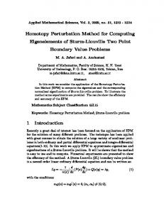
Fig. 1. The averageof all boom (upper) and mast (lower)stream-

wisevelocityspectrausedin the analysisnormalized by u2,.The circles are the average of the uncorrected spectra as measured during HEXMAX; the solid lines are the averagesof the spectra after correction. The labels indicate the principal cause for

Becauseof problemswith the dew point temperature sensors,we were unable to obtain in situ Lyman-a calibrations. Post-HEXMAX calibration of our Lymaa-as was accore- deviationfrom a-2/3 slope.

EDSONET AL.' INERTIAL-DISSIPATION METHOD

Hamming window obtained in this manner agreedwith the

resultsdescribedabove(seeFairall et al. [1990]and Edson et al. [•000a]for details).

10,693

w'T'= w'--r•, -0.51Tw'q' +• where we define

The corrected and uncorrectedstreamwisevelocity spec-

aU

tra averaged overall runs(normalized by u•.) aregivenin Figure 1 for the boom and mast sonicanemometers.In both devicesthe samplingfrequencyis 18.83 Hz, suchthat exten-

sionof the-2/3 slope(in thisrepresentation) past9.42Hz is purely a result of our corrections. On the basis of our theo-

reticalinvestigation,the •dditionaldeviationsfrom the -2/3 line are principally due to the effectsof finite samplingtime at 4 Hz, a combination of finite sampling and spatial and temporM averagingeffectsbetween4 and 8 Hz, and spatial

and temporalaveragingeffects(as well as the appliedoutput filters)beyond8 Hz. Additionaluncertainties causedby the sonichardware(e.g., hard-wiredfilters and internalcoordinateconversions) beginto affectthe spectraaround10 Hz. Therefore in the analysis that follows, the upper limit of the sonic frequenciesused in our corrected estimates is 8 Hz.

Sonic Temperature The T, values from the cold-wire sensors are not reliable

becausethe wires were contaminatedby sea salt [Fairall et al., 1990]. Temperaturecontaminationby salt particlesresidingon small temperature sensorswas discussedby

Schmittet al. [1978].In light of thisproblem,weput a good deal of effort into obtaining turbulence measurementsfrom the sonic thermometer. Temperature corrections are also required for the Kaijo Denki sonicsused during HEXMAX becauseof velocity crosstalk and time averagingcausedby the nonsimultaneousemissionof the acousticpulsesused to compute the temperature signals. The complete processis describedin detail by Larsen et

al. (1991). Briefly,the inertial-dissipation methodcan be usedwith the sonicthermometerif the temperature variance spectrum is correctedfor the contamination by velocity fluctuations associatedwith the time delay betweensamplingof the opposingacousticpropagation paths. Scale analysison the error terms has shown that

the corrections

to the fre-

quency spectra can be approximated by

=

(13a)

w'T•'. = w . + •-w'•'

(a3)

as the sonicvirtual temperature covariance. Computationof Structure Function Parameters

Once the measuredspectra have been correctedfor the

variouseffectsdescribedabove,the structurefunctionparametersare obtainedfrom the frequencyspectraby using

equations (6) and(7), andTaylor'shypothesis (i.e.,assuming k•(k)= fS(f) with k = 2orf/U) as

C•=4(-•) 20r 2/a 1• fS/aSx(f) Px•

(14)

wherethe summationis overthe measured discretespectral pointsbetweenspecifiedupperand lowerlimits of f. The factorPx includestermsthat correctfor anisotropyandinaccuracies in Taylor'shypothesis in the inertial subrange givenby Wyngaardand Clifford[1977].In our analysiswe usedf = 2, 4, 6 Hz for the mast sonic;f = 4, 6, 8 Hz for the boom sonic;and f •- 6, 8, 10, 12, 14 Hz for all other devices.As statedin the precedingsubsection, thesefrequencies werechosento minimizethe uncertaintycausedby the spectralcorrections,while maintainingconfidence that the -5/3 law of the inertialsubrange remainsvalidfor our streamwisevelocityspectra. This confidenceis basedon the

fact that all valuesof the normalized frequency fz/U used in our analysisare greaterthan 1.5 underpredominantly unstable conditions [e.g.,Panofsky andDutton,1984]. 4. DIMENSIONLESS

STRUCTURE FUNCTION

PABAMETER

ANALYSIS

Preliminaryresultsconcerning the empiricalstructure

function parameters werepresented by Fairallet al. [1990] and Edsonet al. [1990b].Sincetheir submissions, we completedourdetermination ofthepropercalibration andspectral correction asdescribed above.Theimproved accuracy warrantsa morecompleteanalysisof the empiricalstructure

(12a)

S,(f) ? S,o(f)sec2(2orfrp)

functionparametersthan that givenpreviously.Therefore the set of dimensionless structurefunctionparameters derived in this sectionrepresentsthe consensus of the HEX-

(12b) MAX inertial-dissipation group,andsupersedes anyprevi-

whereSx(f) is the frequencyspectrum,rp is the time interval betweenpulses,a is equalto 2TIC whereC is the speed of sound, and the subscript s denotes the measured sonic

ous results.

The followingestimationsof the empiricalfunctionsare

foundusing(8) by examining C•z•/a/z•.versus f. The

near-neutral conditions experienced during value. Equation(12a) givesthe sonicvirtual temperature predominantly entirelynewparamspectrum from which we obtain the sonic virtual temper- HEXMAX makeit difficultto suggest ature scalingparametermentionedabove. Equation(12b), eterizationsof fz(f). However,by comparingpreviousesthe correctionto the streamwisevelocity spectra due to this time delay, has been included to showthat temperature contamination on thesemeasurementsis negligible. The inverse cosineterm reflectsthe averagingof the variable at the two shootingtimes and has been included in our calculation of the filter function.

timates, we can make some claims about the behavior of

thesefunctionsand their valueswithinthe stabilityrange -0.75 _• f _• 0.2, whichwe believewill clarify someof the ambiguity in the choiceof the functions mentioned above. Stability Dependence

The cospectrumis not affectedby the differencein shootIn this sectionwe usein all the scalingparametersthe ing times,but the covaxiance of sonictemperatureand ver- valuesof u, determined from the boom covarianceestimates. tical velocitymuststill be corrected for the normalvelocity The subscript c denotes the value of u, corrected for the

andmoisturecontamination [Schotanus et al., 1983]:

boomdistortionas described in section6. The stability

10,694

EDSON ET AL.: INERTIAL-DISSIPATIONMETHOD

parameter • is defined using the boom scalingparameters

foundin the majorityof pastfieldexperiments [e.g.,Dyer, 1974;Dyer and Bradley,1982;HSgstrSm, 1988],with the notableexception of the 1968KansasExperiment. In light z•gT.•, (15a)of this we modifythe dimensionless profilefunctionswhen necessary usingthe approach of HSgstrSm [1988],wherewe and the scalingparameters are found from our covariance furtherassume that the ratioof the eddyviscosity to eddy measurements

conductivityK,,/Kh is equalto 1 at • = 0. Thesefunctions

u.c = (-w--•7u')•

for unstable conditions are identified as follows:

(15b)

ModifiedBusinger et al. [1971](MB71)

q, = -(w'-•)/u,c

(15d)

where(15c)wasfoundusing(13b). Usingthe sonicvirtual temperatureflux in (15a) to estimatethe buoyancyflux in-

•bm(() -- (1- 20.3•)-•/'

(183)

•b•,(•)-- •bh(•)----(1-- 12.2•) -•/2

(18b)

ModifiedDyer [1974](MD74)

•bm(•)= (1 - 16•)-•/'

(19a)

•bw(() ----•bh(•)----(1-- 16•)-•/2

(19b)

troducesa negligibleoverestimationin of at most 3% for the conditionsthat we encounteredduring HEXMAX. To minimize the calibration uncertainty of the Lyman-c•s

in ourdetermination ofCq2Z213/q. 2,wepaired thehumidityvelocity covariancewith the spectral estimate derived from the same Lyman-c•. Note that the sonic temperature data are not included

in this section

because the correction

Dyer andBradley[1982](DB82)

to

= (] - 2s()-,/,

(20.)

the temperaturespectradescribedby Larsenet al. (1991) requiresone to specify the forms of the empirical functions and constantsbeforehand.Therefore usingthesespectrain the analysis would bias the results.

•b•,(•) ---•bh(•) ---(1-- 14•)-•/2

Followingrecentdevelopments in the literature[Andreas, ModifiedWebb[1982](MW82) 1987; Hill, 1989], we assumethat the scalar Kolmogorov constantsand similarity functionsare identical. We begin our analysisby testing which of the previousfindingsgives the best agreementwith our over-oceanmeasurements.The

•b,•(•)= 1 + 4.5•

-• •_0.032

[1971](WC71),

f,(•) ---4.2(1+ 0.51e I

e •_0

(21a)

•,•(•) = (25.25 I • I)-t[] + (190.5•) -1] 0.032 < -• • 0.27 (21b)

first set of functions is drawn from the dimensionless dissi-

pation function measuredover land by Wyngaardand Cotd

(20b)

•.•(•) = 0.43I •

+ (190.5•) -•] 0.27< -• _•0.54 (21c)

(16a)

d',•,(•) = 0.37 I • I-t[] + (190.5•) -•] 0.54 < -• (21d) f,(•) = 4.2(1+ 2.5•3/5) • •_0

(16b)

andthe scalarfunctiongivenby Wynaard[1973](W73)

f•,(•) = fq(•)= 4.9(1-7•)-2/3 • _•0

,,(()

= ,.(()

-•

_• 0.27

(21e)

(16c) =

f•,(f) = fq(f)-- 4.9(1+ 2.4f2/a) f •_0

=

=

0.27 0

Set

z

Runs, N

Range of•

•