NASA/CR—1998-208687
A Summary of Validation Results for LEWICE 2.0 William B. Wright Dynacs Engineering Company, Inc., Brook Park, Ohio
December 1998
AIAA–99–0249
The NASA STI Program Office . . . in Profile Since its founding, NASA has been dedicated to the advancement of aeronautics and space science. The NASA Scientific and Technical Information (STI) Program Office plays a key part in helping NASA maintain this important role.
•
CONFERENCE PUBLICATION. Collected papers from scientific and technical conferences, symposia, seminars, or other meetings sponsored or cosponsored by NASA.
The NASA STI Program Office is operated by Langley Research Center, the Lead Center for NASA’s scientific and technical information. The NASA STI Program Office provides access to the NASA STI Database, the largest collection of aeronautical and space science STI in the world. The Program Office is also NASA’s institutional mechanism for disseminating the results of its research and development activities. These results are published by NASA in the NASA STI Report Series, which includes the following report types:
•
SPECIAL PUBLICATION. Scientific, technical, or historical information from NASA programs, projects, and missions, often concerned with subjects having substantial public interest.
•
TECHNICAL TRANSLATION. Englishlanguage translations of foreign scientific and technical material pertinent to NASA’s mission.
•
•
•
TECHNICAL PUBLICATION. Reports of completed research or a major significant phase of research that present the results of NASA programs and include extensive data or theoretical analysis. Includes compilations of significant scientific and technical data and information deemed to be of continuing reference value. NASA’s counterpart of peerreviewed formal professional papers but has less stringent limitations on manuscript length and extent of graphic presentations. TECHNICAL MEMORANDUM. Scientific and technical findings that are preliminary or of specialized interest, e.g., quick release reports, working papers, and bibliographies that contain minimal annotation. Does not contain extensive analysis. CONTRACTOR REPORT. Scientific and technical findings by NASA-sponsored contractors and grantees.
Specialized services that complement the STI Program Office’s diverse offerings include creating custom thesauri, building customized data bases, organizing and publishing research results . . . even providing videos. For more information about the NASA STI Program Office, see the following: •
Access the NASA STI Program Home Page at http://www.sti.nasa.gov
•
E-mail your question via the Internet to
[email protected]
•
Fax your question to the NASA Access Help Desk at (301) 621-0134
•
Telephone the NASA Access Help Desk at (301) 621-0390
•
Write to: NASA Access Help Desk NASA Center for AeroSpace Information 7121 Standard Drive Hanover, MD 21076
NASA/CR—1998-208687
A Summary of Validation Results for LEWICE 2.0 William B. Wright Dynacs Engineering Company, Inc., Brook Park, Ohio
Prepared for the 37th Aerospace Sciences Meeting and Exhibit sponsored by the American Institute of Aeronautics and Astronautics Reno, Nevada, January 11–14, 1999
Prepared under Contract NAS3–98022
National Aeronautics and Space Administration Lewis Research Center
December 1998
AIAA–99–0249
Acknowledgments
The authors would like to thank the NASA Lewis Icing Branch for their continued support of this research, both financially and for their help with this report. Special recognition goes to the researchers who generated the experimental data included in this report, to Dr. Mark Potapczuk for his insights into this work and especially to Tammy Langhals for digitizing all of the experimental ice tracings in this report.
Available from NASA Center for Aerospace Information 7121 Standard Drive Hanover, MD 21076 Price Code: A03
National Technical Information Service 5285 Port Royal Road Springfield, VA 22100 Price Code: A03
A Summary of Validation Results for LEWICE 2.0 William B. Wright * Dynacs Engineering Co., Inc.
I. Abstract A research project is underway at NASA Lewis to produce a computer code which can accurately predict ice growth under any meteorological conditions for any aircraft surface. This report will present results from version 2.0 of this code, which is called LEWICE. This version differs from previous releases due to its robustness and its ability to reproduce results accurately for different point spacing and time step criteria across several computing platforms. It also differs in the extensive amount of effort undertaken to compare the results in a quantifiable manner against the database of ice shapes which have been generated in the NASA Lewis Icing Research Tunnel (IRT). The complete set of data used for this comparison is available in a recent contractor report1. The result of this comparison shows that the difference between the predicted ice shape from LEWICE 2.0 and the average of the experimental data is 7.2% while the variability of the experimental data is 2.5%.
II. Introduction The Icing Branch at NASA Lewis has undertaken a research project to produce a computer code capable of accurately predicting ice growth under a wide range meteorological conditions for any aircraft surface. The most recent release of this code is LEWICE 2.0. which will be documented in the new user manual.2 This report will not go into the details of the capabilities of this code, as those features are welldescribed by the user manual. The purpose of this paper is to present results from the complete set of data used for validation of this code as well as identify and assess criteria which are used to validate the NASA icing codes. The measurement technique used in this report are not necessarily the only criteria which can be used for validation but they represent one possible path. The process for validation of an icing code is quite challenging and consists of many steps, one of which is the comparison of code results to some known solution whether experimental or analytical. This testing * Senior Member, AIAA
activity is complicated by the fact that no predefined acceptance criteria have been identified. To date, previous evaluation of the performance of ice prediction codes has been based on subjective judgements of the visual appearance of comparisons between ice shapes generated by the code and ice shapes measured in an experimental facility3-10. In order to accurately determine the capabilities of a prediction code it is necessary to develop quantitative measures for assessing the similarity between two ice shapes. The measurement used to make the comparison should be based on the characteristics considered most important for the purposes of the simulation process. For example, design of a thermal ice protection system may dictate that icing limits, accumulation rates, and total collection efficiency are the most important parameters to be simulated while certification of a wing for flight with an ice accretion may require that the performance characteristics of the ice shape be modeled accurately. In past reports11-16, LEWICE has been compared to shapes created in the NASA Lewis Icing Research Tunnel (IRT). While the qualitative comparisons have been favorable, they do not demonstrate a validation process that quantitatively determines the accuracy of an ice prediction code. Comparisons are made in this paper using a large subset of the data which has been generated in the IRT. The test entries which were not used for comparison represent ice shapes from proprietary tests or those tests for which the ice shapes were not digitized. The results are examined from a more quantitative approach than has been undertaken in previous efforts. Measured quantities are horn length, horn angle, stagnation point thickness, ice shape cross section area and icing limits. This paper will define the differences between experimental ice shapes and LEWICE 2.0 as well as the differences between two experimental ice shapes, where applicable. Due to the large number of shapes, an aerodynamic performance analysis was not performed at this time. The report is divided into four sections. The first section will provide a brief description of LEWICE and the LEWICE 2.0 model. The second section will
1 American Institute of Aeronautics and Astronautics
Copyright ©1998 by the American Institute of Aeronautics and Astronautics, Inc. No copyright is asserted in the United States under Title 17, U.S. Code. The U. S. Government has a royalty-free license to exercise all rights under the copyright claimed herein for Governmental Purposes. All other rights are reserved by the copyright owner.
have been minimized and demonstrated; that the code inputs and outputs are consistent and easy to understand; that the structure and documentation within the code makes it readily modifiable to those outside the standard LEWICE development team; and that the code has been validated in a quantified manner against the largest possible amount of experimental data. This last statement forms the basis of the comparisons in this report.
provide a description of the experimental data presented in this report. The third section will describe the quantitative parameters chosen and how they were measured. The fourth section presents results of the quantitative comparison. Comparison of LEWICE 2.0 with the experimental average is presented as well as the comparison of individual experimental ice shapes against the average. Spanwise variability and repeatability variability are presented as well as the variability due to the technique used by the researcher to trace the ice shape.
IV. Description of the Experimental Data
III. LEWICE 2.0
The experimental data described in this paper are the result of a wide variety of tests performed in the NASA Lewis Icing Research Tunnel (IRT) in recent years.17-24 Seven airfoils were selected for this comparison. These airfoils and the accompanying ice shapes represent the complete set of publicly available data which has been generated in the IRT and digitized for single element airfoils. There is some data available on multi-element airfoils, but it was considered to be an insufficient amount for validation purposes. There are a total of 400 IRT runs analyzed for this validation report, of which 169 are repeats of previous runs in the IRT. There are 442 digitized tracings at off-centerline locations for a total of 842 experimental ice shapes. The first airfoil is a modified NACA230XX series airfoil with a slight spanwise taper and sweep. At the mid-span of the test section, the thickness is 14.5% chord and increases in thickness from the floor to the ceiling of the test section. In this paper, it is listed as a modified NACA23014 airfoil, as the thickness is closer to 14% at the lower end of the model. This data was originally presented in references 17-20. The cross-section at the mid-span of the test section is given in Figure 1. The database for this airfoil is comprised of 62 IRT runs, of which 22 are repeats of previous conditions. Due to the spanwise variation of the model, only 8 tracings have been digitized at offcenterline locations for a total of 70 ice shapes. The second airfoil listed is shown in Figure 2. It is representative of a Large Transport Horizontal Stabilizer and is listed with the abbreviation LTHS. This data was originally reported in reference 17. There are 28 IRT cases, of which only one is a repeat of a previous run. There are 52 tracings digitized at offcenterline locations for a total of 80 ice shapes.
The computer code LEWICE embodies an analytical ice accretion model that evaluates the thermodynamics of the freezing process that occurs when supercooled droplets impinge on a body. The atmospheric parameters of temperature, pressure, and velocity, and the meteorological parameters of liquid water content (LWC), droplet diameter, and relative humidity are specified and used to determine the shape of the ice accretion. The surface of the clean (un-iced) geometry is defined by segments joining a set of discrete body coordinates. The code consists of four major modules. They are 1) the flow field calculation, 2) the particle trajectory and impingement calculation, 3) the thermodynamic and ice growth calculation, and 4) the modification of the current geometry by addition of the ice growth. LEWICE applies a time-stepping procedure to “grow” the ice accretion. Initially, the flow field and droplet impingement characteristics are determined for the clean geometry. The ice growth rate on each segment defining the surface is then determined by applying the thermodynamic model. When a time increment is specified, this growth rate can be interpreted as an ice thickness and the body coordinates are adjusted to account for the accreted ice. This procedure is repeated, beginning with the calculation of the flow field about the iced geometry, then continued until the desired icing time has been reached. LEWICE 2.0 is different from its predecessors not through wholesale changes in the physical models but rather through an extensive effort to adjust, test and document the code to ensure: that the code runs correctly for all of the cases shown; that the quality of output is maintained across platforms and compilers; that the effects of time step and spacing
2 American Institute of Aeronautics and Astronautics
tions of the ice shape are traced and digitized in this manner. There are several steps within this process which can potentially cause experimental error. Those which can be quantified by the current technique are the spanwise variability, the repeatability error, and errors involved in the tracing technique.
The third airfoil in the database is representative of a business jet airfoil and given the designation GLC305. It is shown in Figure 3. This data was originally reported in reference 17. There are 84 IRT cases, of which only eight are repeats of a previous run. There are 36 tracings digitized at off-centerline locations for a total of 120 ice shapes. The fourth airfoil in the database is the NACA0012. This airfoil has been used in several test entries over the years17, 25, 26 in order to document the uniformity and repeatability of the IRT, especially after the tunnel had undergone modifications which could potentially alter the tunnel calibration. This airfoil is shown in Figure 4. The data from this airfoil encompasses the highest number of ice shapes which have been created in the IRT. There are 183 IRT cases, of which 126 are repeats of a previous run. There are 307 tracings digitized at off-centerline locations for a total of 490 ice shapes. The fifth airfoil in the database is a modified NACA4415 airfoil and is shown in Figure 5. This airfoil is representative of an airfoil used in past regional aircraft design. The data was originally presented in reference 19. There are 29 IRT cases, of which 11 are repeats of a previous run. There are 39 tracings digitized at off-centerline locations for a total of 68 ice shapes. The sixth airfoil presented is an NLF-0414 airfoil which is representative of a laminar flow design for general aviation. It is shown in Figure 6. This data comes from a very recent test in the IRT21. Due to time constraints, only eight cases from this test entry have been digitized and analyzed for this comparison. Additional test points from this airfoil will be included for future validation efforts. The last airfoil entry in the database is for a NACA0015 airfoil used for scaling studies. This airfoil is shown in Figure 7. This data is also from a very recent test entry in the IRT23. Again due to time constraints only six cases were processed for this effort, one of which is a repeat case. The data is taken in the IRT by cutting out a small section of the ice growth and tracing the contour of the ice shape onto a cardboard template with a pencil. The pencil tracing is then transformed into digital coordinates with a hand-held digitizer. Recently, a flat-bed scanner with digitizing software has been available to accelerate the data acquisition process. For any given IRT test run, up to five spanwise sec-
Spanwise Variability Except for the NACA23014(mod) model, all of the models used for this comparison are two-dimensional models. This means that they have a constant cross-section in the spanwise direction and are mounted in the test section without any sweep angle. Even with a two-dimensional model, the ice shape produced in the tunnel will have some spanwise variability due to the random nature of the ice accretion process. One means which has been used in the IRT to assess this variability is to take ice tracings at several spanwise sections. In the reports mentioned previously, the variability was assessed in the same qualitative manner as comparisons of predicted ice shapes. One technique often used was to visually inspect the ice shape and the cardboard tracings for similarity in the spanwise direction. The shapes may also be digitized at each tracing location and plotted to assess the variability. This report applies the quantitative scale described in section V for assessing both LEWICE predictions and the variability of the test condition. In both cases, the reported difference will be the difference between a measurement on a given ice shape and the average of the experimental measurements for that condition.
Repeatability Several tests in the IRT have also assessed experimental error by running the same flow and spray conditions for the same airfoil multiple times. Cases processed for this validation effort have been repeated by the researcher by immediately running the same condition again, by running the same condition on a different night than the original test and by running the same condition in a different test entry with the same model. In the past for each of these cases, the researcher would apply the same qualitative assessment of the repeatability of the condition. This study will apply the quantitative scale described in section V for assessing LEWICE predictions for
3 American Institute of Aeronautics and Astronautics
assessing the quantitative repeatability of ice shapes in the IRT.
tal and predicted ice shapes. This methodology has been incorporated into a computer code called THICK which calculates and outputs the parameters described. This code was created in order to process the large number of ice shapes presented in this report. This program reads two geometry files: one for the clean airfoil and one containing an ice shape. This code will also be documented more thoroughly in the LEWICE 2.0 User Manual2. The following sections describe the calculations made by the THICK program.
Tracing Technique There are several potential errors involved in the ice tracing and digitization process which in the past have been difficult to quantify. Some of these errors are the quality of the template, the technique used by the researcher to trace the ice shape, and the digitization process. The template is a rectangular piece of cardboard which has the contour of the airfoil cut into it. This is illustrated in Figure 8. As can be seen from this figure, if the ice shape extends beyond the dimensions of the template, it cannot be traced. Additionally, in the past the contour of the airfoil was not always cut precisely into the template so the template may not have fit squarely onto the airfoil. More recent tracing techniques use registration marks to ensure precise fit. The technique used by the researcher also may have an effect on the final digitized ice shape. The template may not be placed squarely on the airfoil or the researcher may only trace the tops of ice feathers or not trace feathers at all, as the feather may break off due to the pressure applied by the pencil. The researcher may not always trace a single continuous line for the ice shape, making the digitalization process more difficult. In order to assess these potential errors, researchers may trace the ice shape more than once or have more than one person trace the same shape. These tracings were then compared in the same qualitative manner as used for spanwise variability and repeatability. Multiple tracings of the same ice shape are rarely performed in the IRT and even more rarely are both tracings digitized. Those which have been digitized are included in this report to provide a more quantitative assessment of the errors involved in the data acquisition process. It will be shown that despite the problems listed here, the quantitative errors due to tracing issues are minor in comparison to other sources of error.
Calculation of Ice Thickness The ice thickness distribution for both experimental ice shapes and LEWICE ice shapes is determined by using a combination of two measurement techniques. The thickness is first measured by calculating the minimum distance from each point on the ice shape to a point on the clean surface. If the distribution of points on the clean surface is sufficiently concentrated, this procedure will provide a good approximation to the actual ice thickness. For this effort, each clean airfoil geometry contained over 5000 points to ensure the quality of the calculation. An approach using the unit normal from the ice shape or from the surface will fail to determine ice thickness at every location on complex ice shapes. This is illustrated in Figure 9. As seen in this figure, the unit normal from the surface diverges outward. Even for a geometry with over 5000 surface points, a unit normal approach could not accurately capture thickness on the large and complex ice shapes presented in this report. This is especially true of experimental ice shapes which have a large amount of detail. The minimum distance approach will very accurately determine large ice thicknesses. For very small ice thicknesses, however, the accuracy is lessened as the thickness nears the resolution of the surface geometry. This is illustrated in Figure 10. The procedure used is to first calculate the thickness using the minimum distance approach. When this thickness becomes less than the segment length of either the iced or clean surface, it is then recalculated using the unit normal approach. Using the approach described, a unique ice thickness is determined for each point on the ice shape. At each point on the clean surface, however, it is possible to have regions where there is no recorded thickness or for a
V. Description of Comparison Method This section describes the methodology used to make the quantitative measurements on experimen-
4 American Institute of Aeronautics and Astronautics
recorded. This thickness is often termed the “stagnation point thickness”, but the aerodynamic stagnation point is not necessarily at this location. In this report, the term “min. leading edge thickness” is used instead. For a rime ice shape, the term “horn” does not apply, nor are there two distinct maxima to record. For this case, only the max. ice thickness and the x,y location at this maxima are recorded.
point to have more than one thickness value. This is illustrated in Figure 11. In the first case where there is no thickness recorded, a thickness value at the clean surface can be interpolated from the values which have been obtained. In the second case where more than one value exists, the maximum ice thickness value is recorded.
Determination of Icing Limits Determination of Max. Thickness Angle
The upper and lower limits of ice accretion for both experimental shapes and LEWICE shapes are easily found from the ice thickness distribution. They are located at the points on the clean airfoil where the ice thickness first changes from zero as measured from the trailing edge. Experimental ice shapes may have sections where parts of the ice (ice feathers) are isolated from the main ice shape. This definition extends the icing limit to include this section of the ice shape. It should also be noted that the definition used in this report for icing limit is distinct from the impingement limit, which only refers to the extent of water collection on the airfoil. Both the wrap distance from the leading edge and the x-distance are recorded for each icing limit. The icing limits are illustrated in Figure 12 on a sample ice shape. Figure 13 shows the icing limits on the ice thickness plot for this ice shape.
The max. thickness alone does not adequately capture all of the necessary quantitative attributes desired. Some indication of where that max. thickness occurred is also desirable. For this effort, the x,y locations at the max. thickness were recorded for each ice shape, both experimental and for LEWICE. An angle at the max. thickness is then calculated. The reference location for all cases is the center of the inscribed circular cylinder at the leading edge for each airfoil. This is illustrated in Figure 16. Again note the terminology of “max. thickness angle”. As discussed earlier, not all ice shapes have a classic glaze ice “horn” but every ice shape has a max. thickness. Where a glaze ice horn does exist, however, this measurement does define the “horn angle”.
Determination of Maximum and Minimum Thicknesses
Determination of Ice Area The iced area calculated for this report is not a true area. A more simplified calculation was performed by integrating the ice thickness calculated with respect to the wrap distance, as given by Equation 1. The approach used is valuable for quantitatively assessing ice shape features such as horn width which are not included in the other parameters.
Three ice thicknesses were selected for the quantitative analysis, the upper surface max. thickness, the lower surface max. thickness and the min. thickness between these two maxima. These thicknesses are illustrated in Figure 14. In this illustration, the upper surface and lower surface maxima clearly correspond to the classic definition of a glaze ice horn. For other conditions this may not be the case, hence the use of the term “max. thickness” rather than “horn thickness”. This differentiation is usually found on smaller ice shape for which the max. thickness is not easily seen. This is illustrated in Figure 15. For the upper surface and lower surface max. thickness, the x,y locations at the maxima are also saved for calculation of a max. thickness angle. The min. thickness between the two maxima is also
A =
∫ t ds
(1)
For the large number of points used on the clean surface, the calculation given is a reasonable approximation of area. Three areas are recorded: the total iced area, the lower surface area and the upper surface area. The lower surface area is defined as the ice area below the leading edge and the upper surface ice area is calculated by subtracting the lower
5 American Institute of Aeronautics and Astronautics
determined by equating the lift coefficient predicted by LEWICE on the clean airfoil for a given case with the lift coefficient on the airfoil at the angle of attack run in the tunnel.
surface value from the total. For complex ice shapes where the ice thickness is multiply defined as is shown in Figure 11, this method for calculating ice area will result in an overstatement of the actual ice area.
VII. Quantitative Results
VI. Procedure for the LEWICE Runs
For each of the 842 experimental ice shapes and 231 predicted ice shapes, the quantitative measurements described in a previous section were taken and then entered into a Microsoft Excel® spreadsheet. A description of the exact contents of this spreadsheet is given in the validation report1. In that contractor report, each of the 231 ice shapes is plotted against the tunnel centerline ice shape for that condition. The ice thickness distribution is also plotted. This paper will provide a summary of results of the quantitative comparison between the LEWICE predicted shape and the experimental average as well as the comparison of individual experimental ice shapes to this average. In each case, the experimental average for a given quantity is the average of all experimental ice shapes at that condition. Repeat runs and off-centerline measurements are averaged with the centerline value to arrive at this measurement.
There are 231 cases which were run with LEWICE for this validation study. This is the complete set of unique conditions, as 169 of the 400 test entries are repeat conditions. All of the cases run for this validation test were performed using the same procedure on a Silicon Graphics Indigo2 to ensure the consistency of the LEWICE predictions. It is well known that a user of an ice accretion code may alter the ice shape prediction by varying the time step and/ or the panel spacing until a desired prediction is achieved. This procedure was not followed for these validation runs. For every run, the point spacing was fixed at a value of 4*10-4 (dimensionless). This was the smallest value which could be used for the array sizes in the program. The time step for all runs was 1 minute for cases where the accretion time was 15 minutes or less. For longer runs, an automated procedure was implemented based on accumulation parameter. When the accumulation parameter exceeded 0.01 for that time step, a new time step was started. The number of time steps is calculated internally in the program by Equation 2. ( LWC ) ( V ) ( Time ) N = -------------------------------------------------( chord ) ( ρ ice ) ( 0.01 )
Icing Limits The icing limits are the chordwise locations on the ice shape on the upper and lower surface where the ice shape merges with the airfoil. Both the wrap distance from the leading edge and the x-distance are recorded for each icing limit. The results presented here are for the wrap distance values. Figure 18 shows the results of these measurements for both the experimental ice shapes and for LEWICE. These results are presented as a percentage of chord in order to normalize the results for different cases. This figure shows that the experimental variation in the lower icing limit is 2% of chord while the LEWICE result lies within 6% of chord from the experimental average value. This result uses the absolute error for each case in order to compute the average. Contrary to popular belief, in the majority of cases LEWICE underpredicts rather than overpredicts the icing limit as compared to the experimental data. This result can likely be attributed to the use of a monodispersed drop size when obtaining the predicted result.
(2)
where LWC = liquid water content (g/m3) V = velocity (m/s) Time = accretion time (s) chord = airfoil chord (m) ρice = ice density = 9.17*105 g/m3 The variability of LEWICE results for various time steps and point spacings is discussed in the section on Numerical Variability in the validation report1. The LEWICE cases had an additional correction due to the use of a potential flow code for the flow solution. As illustrated in Figure 17, a potential flow code will overpredict lift coefficient especially at high angles of attack. To compensate for this, all LEWICE cases were run using a corrected angle of attack. This is
6 American Institute of Aeronautics and Astronautics
Max. Ice Thickness (Horns)
leading edge. This angle was measured for all ice shapes whether or not they fit the classical definition of having a glaze ice horn. Many experimental ice shapes were in the form of distributed roughness with several peaks which can cause a large amount of scatter in the experimental results shown. Figure 21 shows the variation in max. thickness angle for LEWICE and for the experimental categories described earlier. Results are presented in degrees. This figure shows that the variation in the experimental data is 6 degrees for the upper angle, 10 degrees for the lower angle and 13 degrees for the difference between these angles. The LEWICE difference from the experimental average are 16 degrees for the upper angle, 30 degrees for the lower angle and 33 degrees for the angle difference.
The details of the ice thickness calculation were presented in the section on Description of Comparison Method. As discussed in this section, the measurement of a max. thickness is not necessarily the thickness of a glaze ice horn. Where the ice shape does have a glaze ice horn, the max. thickness does give the horn thickness. In order to compare different conditions with different chord lengths and accretion conditions, the individual ice thicknesses were nondimensionalized by the maximum accumulation thickness as given in Equation 3. ( LWC ) ( V ) ( Time ) t max = --------------------------------------------ρ ice
(3)
Figure 19 shows the dimensionless difference in ice thickness for the three ice thickness measurements made in this report. Results are presented for the variation of tunnel repeatability, spanwise variability, tracing error as well as for the overall experimental error and for LEWICE. This figure shows that the max. thicknesses can be measured to within 5% experimentally and that the average difference for the LEWICE cases is 11% for max. thickness.
Overall Assessment Once the individual measurements are taken for each ice shape, it becomes useful to create an overall assessment of the ice shape prediction. Since each measurement is different, several methods could be used to assess the overall difference between two ice shapes. Eight of the 11 measured values presented in this report have been nondimensionalized. Angles do not have a characteristic measure to use for nondimensionalization, so the three angle criteria are reported in degrees. Since not all of the measured quantities can be nondimensionalized, two overall assessment factors have been calculated. The first overall assessment was determined by an average of the eight individual dimensionless values and the three angle criteria in degrees. The second overall assessment was calculated by using only the eight dimensionless measurements. Figure 22 shows the comparison of the first overall assessment for each of the experimental errors and for LEWICE. This calculation shows an average overall difference of approximately 4.4 for the experimental data base and 12.5 for LEWICE. Since the angle criteria are not dimensionless, these numbers cannot be considered a percent difference. Figure 23 shows the comparison using the second overall assessment. This second calculation shows an average overall difference of 2.5% for the experimental data and 7.2% for LEWICE. The standard deviation is 1.8% for the experimental data and 4% for the LEWICE results. In order to determine if this simple average is a good assessment of the variation, plots
Ice Area The comparison of ice area for the different cases also poses a problem. A fair comparison across the varied conditions and airfoil sizes is difficult. In this report, the area difference has been nondimensionalized by the maximum accumulation thickness given earlier and by the airfoil thickness. It should be noted that the absolute values for ice area are maintained in the Excel® spreadsheet so that the users of this data can make their own comparisons. Figure 20 shows the results for the ice area comparison. Values for the upper surface ice area, lower surface ice area and overall ice area are shown for each of the categories described earlier. This figure shows that the experimental difference in ice area is less than 4% on the scale given while for the LEWICE results the variation is approximately 10%.
Angle at Max. Thickness (Horn Angle) As described earlier, the horn angle was measured with respect to a horizontal line which goes through the center of the inscribed cylinder at the 7
American Institute of Aeronautics and Astronautics
entire database even at the fast processor speeds available now. A comparison of a selected number of these cases is being planned at this time. This comparison would calculate the difference in predicted aeroperformance for a given difference in ice shape, using both experimental ice shapes and predicted ice shapes from LEWICE. For example, this comparison would try to determine if the difference in aeroperformance for two ice shapes which are 10% different is consistently greater than the difference in aeroperformance for two ice shapes which are only 5% different.
were made of the average variation for the experimental shapes and for the LEWICE shapes. Figure 24 shows an example of two ice shapes which are near the overall experimental average. This plot shows the spanwise variability from a data point in the NACA4415(mod) database. The qualitative comparison of these two ice shapes suggests that the overall assessment parameter is a reasonable approximation. Similarly, Figure 25 shows an example which is at the average variation for the LEWICE cases. The qualitative assessment of this comparison also agrees with the overall assessment parameter used.
VIII. Conclusions Improvements to methodology
This report has presented the quantitative comparisons of several geometric characteristics for a database of over 1000 ice shapes. Measurements of icing limit, ice thickness, ice area and horn angle were made for each ice shape. Comparisons were made for the difference in experimental variations such as tunnel repeatability, spanwise variability and tracing errors. Comparisons were also made for the difference between the predicted ice shape from LEWICE and the average experimental value. Comparisons were made for each individual quantitative criteria. An overall assessment was made for the quantitative comparison as well. This comparison shows that based on the overall assessment criteria presented in this report, the variation in the experimental data was 2.5%±1.8% and the LEWICE predicted ice shape differs from the experimental average by 7.2%±4%. The variation due to tracing technique was found to be statistically insignificant. The spanwise and repeat variability were found to be extremely close and at the same low level (2.5%). This may indicate that the variation in ice shape for either measure are a reflection of the chaotic nature of the icing phenomena and are not due to the tunnel dynamics. The LEWICE predictions on the whole are reasonably accurate, with a significant percentage (35%) of cases within the experimental average. The ice shape data and output files from LEWICE which were generated for this report are included on CD-ROMs along with all of the quantitative comparison numbers in a published contractor report1.
The technique used in this report for quantitative comparison of ice shapes represents only one possible path for quantitative validation of code results. Ruff27 proposed an alternate methodology for creating an overall assessment of ice shape prediction. Other methods can also be tested for creating an overall assessment of ice shape prediction. Due to the number of cases in this database, an important consideration is the efficiency at which quantitative measurements can be taken and entered into a spreadsheet for analysis. The current technique used a stand alone utility program to generate the ice thickness distributions. This code was very useful in generating the data needed for this comparison, but the process of transferring the information to the spreadsheet was time consuming. More efficient methods for acquiring the quantitative parameters will be developed in the future. The definition of max. thickness angle used in this report is not the only possible definition. Other definitions could use the chord line of the airfoil instead of a horizontal line. The reference point could be selected as the leading edge of the airfoil or the point on the clean surface where the ice thickness was defined. Due to time constraints, the definition presented in this report was the only one calculated from the ice shapes. It was stated in the introduction of this report that a quantitative analysis is only one facet of the code validation process. Once the comparison of ice shape has been made, it would be useful to quantify the difference in aeroperformance based on the quantitative difference in geometry. This process would be very time consuming to perform on the 8
American Institute of Aeronautics and Astronautics
IX. Acknowledgments
9 Olsen, W., Shaw, R., and Newton, J., “Ice Shapes and the Resulting Drag Increase for a NACA 0012 Airfoil,” NASA TM-83556, Jan. 1983.
The authors would like to thank the NASA Lewis Icing Branch for their continued support of this research, both financially and for their help with this report. Special recognition goes to the researchers who generated the experimental data included in this report, to Dr. Mark Potapczuk for his insights into this work and especially to Tammy Langhals for digitizing all of the experimental ice tracings in this report.
10 Addy, G.E., Potapczuk, M. G., and Sheldon, D., “Modern Airfoil Ice Accretions,” NASA TM (AIAA 97-0174), Jan. 1997. 11 Wright, W. B. and Potapczuk, M. G., “Comparison of LEWICE 1.6 and LEWICE/NS with IRT Experimental Data from Modern Airfoil Tests,” NASA TM (AIAA 97-0175), Jan. 1997.
X. References 1 Wright, W. B. and Rutkowski, A., “Validation Results for LEWICE 2.0,” NASA CR xxxx, Nov. 1998.
12 Wright, W. B. and Bidwell, C. S., “Additional Improvements to the NASA Lewis Ice Accretion Code LEWICE,” NASA TM (AIAA-95-0752), Jan. 1995.
2 Wright, W. B., “Users Manual for the NASA Lewis Ice Accretion Code LEWICE 2.0,” NASA CR to be published, Jan. 1999.
13 Wright, W.B., “Users Manual for the Improved NASA Lewis Ice Accretion Code LEWICE 1.6,” NASA CR 198355,June 1995.
3 Wright, W. B., Gent, R. W. and Guffond, D., “DRA/NASA/ONERA Collaboration on Icing Research Part II - Prediction of Airfoil Ice Accretion,” NASA CR 202349, May 1997.
14 Wright, W.B., Bidwell, C. S., Potapczuk, M. G. and Britton, R. K., “Proceedings of the LEWICE Workshop,” June 1995.
4 Gent, R. W., “TRAJICE2 - A Combined Water Droplet and Ice Accretion Prediction Codes for Airfoils,” RAE TR 90054, 1990.
15 Wright, W.B., “Capabilities of LEWICE 1.6 and Comparison with Experimental Data,” presented at the SAE/AHS International Icing Symposium, Sept. 1995.
5 Hedde, T. and Guffond, D., “Improvement of the ONERA 3-D Icing Code, Comparison with 3D Experimental Shapes,” AIAA 93-0169, Jan. 1993.
16 Wright, W.B., and Potapczuk, M. G., “Computational Simulation of Large Droplet Icing,” presented at the FAA Phase III Meeting, May 1996.
6 Brahimi, M. T., Tran, P., and Paraschivoiu, I., “Numerical Simulation and Thermodynamic Analysis of Ice Accretion on Aircraft Wings,” Centre de Développement Technologique de l’École Ploytechnique de Montréal, C.D.T. Project C159, Final Report prepared for Canadair, May, 1994.
17 Shin, J and Bond, T.H., “Results of an Icing Test on a NACA0012 Airfoil in the NASA Lewis Icing Research Tunnel,” AIAA92-0647, Jan. 1992. 18 Addy, Jr., H.E., Potapczuk, M.G., and Sheldon, D.W., “Modern Airfoil Ice Accretions,” AIAA-970174, January, 1997.
7 Tran, P., Brahimi, M. T., Tezok, F. and Paraschivoiu, I., ”Numerical Simulation of Ice Accretion on Multi-Element Configurations”, AIAA 96-0869, Jan. 1996.
19 Addy, Jr., H.E., Miller, D.R., and Ide, R.F., “A Study of Large Droplet Ice Accretion in the NASA Lewis IRT at Near-Freezing Conditions; Part 2,” NASA TM 107424, May, 1996.
8 Mingione, G., Brandi, V. and Esposito, B., “Ice Accretion Prediction on Multi-Element Airfoils,” AIAA 97-0177, Jan. 1997.
20 Miller, D.R., “Addy, Jr., H.E.,and Ide, R.F., “A Study of Large Droplet Ice Accretion in the NASA 9
American Institute of Aeronautics and Astronautics
Lewis IRT at Near-Freezing Conditions,” NASA TM 107142, Jan., 1996. 21 Reehorst, A., Chung, J., Potapczuk, M. and Choo, Y., “The Operational Significance of an Experimental and Numerical Study of Icing Effects on Performance and Controllability,” AIAA 99-0374, Jan. 1999. 22 Addy, G., IRT Test Entry, Feb. 1998. 23 Anderson, D. IRT Test Entry, June 1996. 24 Chen, S. and Langhals, T., “Experimental Validation on the Modification Techniques Developed for the New Scaling Methods,” AIAA 99-0245, Jan. 1999. 25 Addy, G., IRT Test Entry, Feb. 1996. 26 Bidwell, C. S. and VanZante, J. F., IRT Test Entry, Jan. 1998. 27 Ruff, G. A. and Anderson, D. N., “Quantification of Ice Accretions for Icing Scaling Evaluations,” AIAA 98-0195, Jan. 1998.
10 American Institute of Aeronautics and Astronautics
NACA23014 (mod) Airfoil 12 8
y(in)
4 0 -4 -8 -12 0
10
20
30
40
50
60
70
x(in)
FIGURE 1.
NACA 23014(mod) Airfoil
LTHS Airfoil
y(in)
5
0
-5 0
10
20
30
40
x(in)
FIGURE 2.
LTHS Airfoil
GLC305 Airfoil
y(in)
5
0
-5 0
10
20
30
40
x(in)
GLC305 Airfoil
y(in)
FIGURE 3.
NACA0012 Airfoil
4 3 2 1 0 -1 -2 -3 -4 0
4
8
12
16
20
x(in)
FIGURE 4.
NACA0012 Airfoil
11 American Institute of Aeronautics and Astronautics
24
NACA4415 (mod) Airfoil
12 8
y(in)
4 0 -4 -8 -12 0
20
40
60
80
x(in)
FIGURE 5.
NACA 4415(mod) Airfoil
NLF-0414 Airfoil 6
y(in)
4 2 0 -2 -4 -6 -8
0
8
16
24
32
x(in)
FIGURE 6.
NLF-0414 Airfoil
NACA0015 Airfoil
3 2
y(in)
1 0 -1 -2 -3 0
5
10
x(in)
FIGURE 7.
NACA0015 Airfoil
12 American Institute of Aeronautics and Astronautics
15
40
FIGURE 8.
Example of a Cardboard Template for Tracing Ice Shapes
Surface unit normal can miss large regions of ice.
Ice unit normal does not intersect surface
FIGURE 9.
Limitations of Unit Normal Approach for Ice Thickness
13 American Institute of Aeronautics and Astronautics
Ice Surface
Clean Surface
Unit Normal thicknesses
Minimum Distance thicknesses FIGURE 10. Limitations of Minimum Distance Approach
Some surface locations may not have ice thickness value due to sparcity of points on ice shape.
Multiple ice shape locations can point to the same surface location. FIGURE 11. Corrections to Ice Thickness Distribution
14 American Institute of Aeronautics and Astronautics
Icing Limits on Sample Ice Shape 3
2
y(in)
1
X (upper limit) 0
Wrap Upper Limit Wrap Lower Limit
-1
X (lower limit)
-2
-3 -3
-2
-1
0
1
2
3
4
x(in)
FIGURE 12. Icing Limits on Sample Ice Shape
Icing Limits Using Ice Thickness Plot 3
Ice Thickness (in)
2.5
2
1.5
Lower Ice Limit
1
Upper Ice Limit 0.5
0 -4
-3
-2
-1
0
Wrap distance on Clean Airfoil as Measured from Hilite (in)
FIGURE 13. Icing Limits Using Ice Thickness Plot
15 American Institute of Aeronautics and Astronautics
1
Ice Thickness Values on Sample Ice Shape 3
Ice Thickness (in)
2.5
2
Upper Surface Max. Thickness 1.5
1
0.5
Minimum Thickness between Maxima
Lower Surface Max. Thickness 0 -4
-3
-2
-1
0
1
Wrap distance on Clean Airfoil as Measured from Hilite (in)
FIGURE 14. Ice Thickness Values on Sample Ice Shape
Ice Shape with Peak Thickness but No Discernible “Horn” 2
1
y(in)
0
-1
-2
-3 -1
0
1
2
3
4
5
x(in)
FIGURE 15. Ice Shape with Peak Thickness but No Discernable “Horn”
16 American Institute of Aeronautics and Astronautics
6
Max. Thickness Angle on Sample Ice Shape 3
2
y(in)
1
Max. Thickness Angle (Horn Angle) 0
Center of Inscribed Cylinder at Leading Edge -1
-2
-3 -3
-2
-1
0
1
2
3
4
x(in)
FIGURE 16. Max. Thickness Angle on Sample Ice Shape
Lift Coefficient for the GLC305 Airfoil 1.5
Potential Flow
Lift Coefficient
Naviér-Stokes 1
0.5
0 0
2
4
6
8
10
Angle of Attack (degrees)
FIGURE 17. Example of Lift Overprediction by Potential Flow
17 American Institute of Aeronautics and Astronautics
12
Variation of Icing Limit Compared to Average Experimental Value
% Difference based on chord
100
80
Lower Icing Limit Upper Icing Limit
60
40
20
0 Lewice
Spanwise Variability
Repeatability
Tracing Technique
Exp. Error
FIGURE 18. Variation of Icing Limit Compared to Average Experimental Value
Variation of Ice Thickness Compared to Average Experimental Value
%Difference based on Accretion Rate
100
80 Lower Max. Thickness Upper Max. Thickness LE Min. Thickness
60
40
20
0 Lewice
Spanwise Variability
Repeatability
Tracing Technique
Exp. Error
FIGURE 19. Variation of Ice Thickness Compared to Average Experimental Value
18 American Institute of Aeronautics and Astronautics
Variation of Ice Area Compared to Average Experimental Value
% Difference based on Accretion Rate and Airfoil Thickness
100
80 Lower Surf. Area Upper Surf. Area Total Area
60
40
20
0
Lewice
Spanwise Variability
Repeatability
Tracing Technique
Exp. Error
FIGURE 20. Variation of Ice Area Compared to Average Experimental Value
Variation of Angle at Max. Thickness Compared to Average Experimental Value 100
Angle Difference (degrees)
80
Lower Angle Upper Angle Angle Difference
60
40
20
0 Lewice
Spanwise Variability
Repeatability
Tracing Technique
Exp. Error
FIGURE 21. Variation of Angle at Max. Thickness Compared to Average Experimental Value
19 American Institute of Aeronautics and Astronautics
Overall Ice Shape Variation Compared to Average Experimental Value 100
Overall Difference Factor
80
60
40
20
0
Lewice
Spanwise Variability
Repeatability
Tracing Technique
Exp. Error
FIGURE 22. Overall Ice Shape Variation Compared to Average Experimental Value
Overall Variation of Nondimensional Measurements 100
Overall % Difference
80
60
40
20
0 Lewice
Spanwise Variability
Repeatability
Tracing Technique
Exp. Error
FIGURE 23. Nondimensional Ice Shape Variation Compared to Average Experimental Value
20 American Institute of Aeronautics and Astronautics
Example of Ice Shape Variation at Average %Difference in Experimental Data 10
5
y(in)
Airfoil 31" Span Tracing 36" Span Tracing
0
-5 -5
0
5
10
15
x(in)
FIGURE 24. Example of Ice Shape Variation at Average %Difference in Experimental Data
Example of Ice Shape Prediction at Average %Difference from Experimental Data
2
Airfoil Experiment Lewice
y(in)
1
0
-1
-2
-2
-1
0
1
2
3
4
x(in)
FIGURE 25. Example of Ice Shape Prediction at Average %Difference in Experimental Data
21 American Institute of Aeronautics and Astronautics
5
Form Approved OMB No. 0704-0188
REPORT DOCUMENTATION PAGE
Public reporting burden for this collection of information is estimated to average 1 hour per response, including the time for reviewing instructions, searching existing data sources, gathering and maintaining the data needed, and completing and reviewing the collection of information. Send comments regarding this burden estimate or any other aspect of this collection of information, including suggestions for reducing this burden, to Washington Headquarters Services, Directorate for Information Operations and Reports, 1215 Jefferson Davis Highway, Suite 1204, Arlington, VA 22202-4302, and to the Office of Management and Budget, Paperwork Reduction Project (0704-0188), Washington, DC 20503.
1. AGENCY USE ONLY (Leave blank)
2. REPORT DATE
3. REPORT TYPE AND DATES COVERED
Final Contractor Report
December 1998 4. TITLE AND SUBTITLE
5. FUNDING NUMBERS
A Summary of Validation Results for LEWICE 2.0 WU–548–20–23–00 NAS3–98022
6. AUTHOR(S)
William B. Wright 7. PERFORMING ORGANIZATION NAME(S) AND ADDRESS(ES)
8. PERFORMING ORGANIZATION REPORT NUMBER
Dynacs Engineering Company, Inc. 2001 Aerospace Parkway Brook Park, Ohio 44142
E–11467
9. SPONSORING/MONITORING AGENCY NAME(S) AND ADDRESS(ES)
10. SPONSORING/MONITORING AGENCY REPORT NUMBER
National Aeronautics and Space Administration Lewis Research Center Cleveland, Ohio 44135–3191
NASA CR—1998-208687 AIAA–99–0249
11. SUPPLEMENTARY NOTES
Prepared for the 37th Aerospace Sciences Meeting & Exhibit sponsored by the American Institute of Aeronautics and Astronautics, Reno, Nevada, January 11–14, 1998. Project Manager, Thomas H. Bond, Turbomachinery and Propulsion Systems Division, NASA Lewis Research Center, organization code 5840, (216) 433–3900. 12a. DISTRIBUTION/AVAILABILITY STATEMENT
Unclassified - Unlimited Subject Category: 02
12b. DISTRIBUTION CODE
Distribution: Nonstandard
This publication is available from the NASA Center for AeroSpace Information, (301) 621–0390. 13. ABSTRACT (Maximum 200 words)
A research project is underway at NASA Lewis to produce a computer code which can accurately predict ice growth under any meteorological conditions for any aircraft surface. This report will present results from version 2.0 of this code, which is called LEWICE. This version differs from previous releases due to its robustness and its ability to reproduce results accurately for different point spacing and time step criteria across several computing platforms. It also differs in the extensive amount of effort undertaken to compare the results in a quantifiable manner against the database of ice shapes which have been generated in the NASA Lewis Icing Research Tunnel (IRT). The complete set of data used for this comparison is available in a recent contractor report . The result of this comparison shows that the difference between the predicted ice shape from LEWICE 2.0 and the average of the experimental data is 7.2% while the variability of the experimental data is 2.5%.
14. SUBJECT TERMS
15. NUMBER OF PAGES
27
Aircraft icing
16. PRICE CODE
A03 17. SECURITY CLASSIFICATION OF REPORT
Unclassified NSN 7540-01-280-5500
18. SECURITY CLASSIFICATION OF THIS PAGE
Unclassified
19. SECURITY CLASSIFICATION OF ABSTRACT
20. LIMITATION OF ABSTRACT
Unclassified Standard Form 298 (Rev. 2-89) Prescribed by ANSI Std. Z39-18 298-102