A Survey on Position-Based Routing Algorithms in Wireless Sensor

Algorithms 2009, 2, 158-182; doi:10.3390/a2010158 OPEN ACCESS

algorithms ISSN 1999-4893 www.mdpi.org/algorithms Review

A Survey on Position-Based Routing Algorithms in Wireless Sensor Networks Zhang Jin 1,2*, Yu Jian-Ping 1, Zhou Si-Wang 1, Lin Ya-Ping 1 and Li Guang 2 1

School of Software, Hunan University, Changsha 410082, China National Laboratory of Industrial Control Technology, Zhejiang University, Hangzhou 310027, China E-mails: [email protected]; [email protected]; [email protected]; [email protected] 2

* Author to whom correspondence should be addressed; E-mail: [email protected] Received: 29 October 2008; in revised form: 17 December 2008 / Accepted: 29 January 2009 / Published: 9 February 2009

Abstract: Wireless sensor networks (WSN) have attracted much attention in recent years for its unique characteristics and wide use in many different applications. Routing protocol is one of key technologies in WSN. In this paper, the position-based routing protocols are surveyed and classified into four categories: flooding-based, curve-based, grid-based and ant algorithm-based intelligent. To each category, the main contribution of related routing protocols is shown including the relationship among the routing protocols. The different routing algorithms in the same category and the different categories are compared based on popular metrics. Moreover, some open research directions in WSN are also discussed. Keywords: wireless sensor network, routing, position, flooding, curve, grid, intelligence

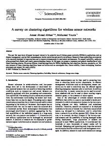
1. Introduction Recent advances of sensor technology have led to the development of micro-sensors with low power and highly integrated functions [1-3]. Each sensor includes sensing unit, processing unit, transmission unit and power unit. Sensors deployed in an application field are organized by themselves to form a virtual organization. The sensing unit measures ambient conditions and transforms them into an electric signal. Then, transmission unit forwards the data to the neighbors. According to multi-hops, the data reaches the base station (sink). The process can be shown briefly as Figure.1.

Algorithms 2009, 2

159 Figure 1. The simple description of WSN [4].

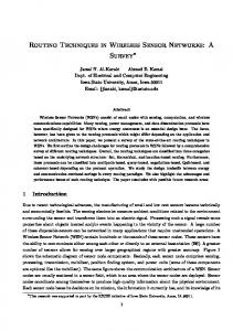
Based on WSN, there are many exciting applications including military applications, environmental applications, health applications, home applications, other commercial applications [1, 5]. In Figure.2, there are two typical applications of WSN. In Figure.2 (a), the special events (such as friendly and enemy forces, equipment and ammunition) in a military application can be monitored. By equipping or embedding equipment and personnel with sensors, vehicle-, weapon-, and troop-status information can be gathered and relayed back to a command center to determine the best course of action. Information from military units in separate regions can also be aggregated to give a global snapshot of all military assets [5]. In Figure.2 (b), an environmental application about forest fire detection is given. Since sensor nodes are randomly and densely deployed in a forest, sensor nodes can relay the warning about fire to the end users taking suitable actions to control the fire spread. Figure 2. Applications based on WSN [5].

(a) Military applications

(b) Environmental applications

In most applications of WSN, it needs to deploy and integrate millions of sensor nodes using radio frequencies systems. Because the sensors may be left unattended for months and even years, effective

Algorithms 2009, 2

160

power-aware methods are needed. The sensor nodes will collaborate with each other to perform distributed sensing and overcome obstacles, such as trees and rocks [1]. These make WSN significantly different from others, such as Ad hoc. Comparing with other networks, these unique characteristics of WSN include several aspects listed as follows [3]: (1) Energy issue is the most important concern. Sensors usually work at unattended area for several years and it is often impractical to recharge or replace a depleted battery. Among all the operations, transmitting and receiving data account for the major portion of the energy [6]. So, energy-aware routing protocol is desired and can significantly prolong the lifetime of WSN. For WSN applications to have reasonable longevity, an aggressive energy-management policy is mandatory. This is currently the greatest design challenge in any WSN applications. (2) Resources for calculating and storing are extremely limited. In order to reduce the sensor cost, sensors are made of simple and low-cost circuits. So, sensor nodes may not have global identification (ID) because of the large amount of overhead and large number of sensors. For example, the Berkley MICA series Motes have 8MHz processors, 128K programmable memory, 4K RAM and 512K flash memory for storage [7]. For the SmartDust nodes, it have 8-bit and 4MHz CPU, 8KB instruction flash memory, 512 bytes RAM, 512 bytes EEPROM, 3500 bytes space for OS code and 10Kilobits/second bandwidth [8]. (3) Sensor nodes are densely deployed. Since the cost of sensors is low and the components are unreliable, the sensors are prone to failure, which makes the topology of WSN change frequently. It is necessary to deploy a large number of sensors to avoid the node failure and cover the monitoring area. (4) The position of individual sensors can not be predetermined. To some typical applications, the monitoring fields could be hostile or dangerous and human can not access it, such as the forest fire detection, chemical pollution, battlefields. So, WSN is randomly deployed in inaccessible terrains or disaster relief operations by an airplane or missile [9]. On the other hand, this also means that sensor network protocols and algorithms must possess self-organizing capabilities. The management and topology control mechanism must be flexible and robust. Considering these unique characteristics, Designing suitable routing protocols in WSN is very challenging due to the inherent characteristics [4]. Though WSN share some common features with MANET (Mobile Ad-hoc NETwork), those protocols proposed for MANET are not well suited for WSN for some reasons. For example, keeping the routing state is not necessary; the collected data has much redundancy; getting the data is more important than knowing which nodes sent the data. Some special routing tactics (such as data aggregation, clustering and data-centric methods) is proposed for routing algorithms in WSN to minimize energy consumption. All routing protocols can be classified based on different standards. According to the network structure, there are flit-based, hierarchical-based and position-based. Considering protocol operation, these routing algorithms can be classified into query-based, negotiation-based, quality of service (QoS)-based. Among these routing protocols, position-based protocols utilize position information to relay the data to the desired regions and show the advantage of energy-awareness. Since, there is no addressing scheme like IP-addresses in position-based routing and they are spatially deployed on a region, position information can be utilized in routing data in an energy efficient way. For instance, if the sensed region is known, the query can be limited only in some particular region to save energy significantly according to the position information of sensor nodes.

Algorithms 2009, 2

161

Although there are some previous efforts on surveying WSN [1, 3, 4, 5, 10, 11], the scope of the survey presented in this article is distinguished from these surveys. The surveys in [1,5,10] addressed the general issues and techniques, such as the physical constraints on sensor nodes, applications, and architectural attributes. The survey in [3,4,11] emphasized on the general routing algorithms. Due to the importance of position information in routing and the availability of many literatures on this topic, a detailed survey becomes necessary and useful. Our work concentrates upon position-based routing algorithms in WSN and the different approaches are described and categorized. The rest of this article is organized as follows. Firstly, we discuss some related works, such as localizing algorithms, coverage and connectivity. Then, a classification and comprehensive survey of position-based routing techniques in WSN is presented. The different routing algorithms of the same category and the different category of position-based routing are compared separately. Finally, some future research directions and open issues related to position information in WSN are also discussed. 2. Related works 2.1 Locating sensors It is obvious that position-based routing protocols require that sensor nodes can somewhat know their position. Though the position information can be known by providing sensors with a GPS unit, it is often unfeasible as the GPS is quite expensive and energy consuming. In order to resolve the locating problem, there are two strategies. One strategy is to equip a limited subset of nodes with a GPS and then derive the location of the other ones by means of other techniques. However, commonly available sensor platforms lack the hardware suitable to acquire location information. The other strategy is that the sensors locate its position based on the relative position to anchors. The localization problem has received considerable attention in the past and recently a number of localization systems have been proposed specifically for sensor networks [12, 13]. Localization algorithms can be divided into two categories: distance-based and distance-free. Distance-based localization algorithms require the sensors to contain hardware for measurements. Distance-free localization algorithms do not use radio signal strengths, angle of arrival of signals or distance measurements and special hardware is not needed. About distance-free localization, various techniques have been proposed for measuring the distances and these techniques can be classified into three subclasses: AOA (Angle of Arrival) measurements, time related measurements and RSS (Received Signal Strength) profiling techniques. (1) AOA measurements make use of the receiver antenna’s amplitude response or phase response to measure the distance. Beamforming is the usual technology and uses the anisotropy in the reception pattern of an antenna. Koks proposed to use a minimum of two stationary antennas with known, anisotropic antenna patterns to cope with the varying signal strength problem [14]. Phase interferometry typically requires a large receiver antenna (relative to the wavelength of the transmitter signal) or an antenna array based on the phase differences in the arrival of a wave front [15]. In [16], Niculescu and Nath have used Angle of Arrival of signals to estimate distances. The accuracy of AOA measurements is limited by the directivity of the antenna, shadowing or by multipath reflections. Another class of AOA measurement methods is based on s subspace-based algorithms, which require a multi-array antenna in order to form a correlation matrix using signals received by the array. The most

Algorithms 2009, 2

162

well known methods include MUSIC (multiple signal classification) [17] and ESPRIT (estimation of signal parameters by rotational invariance techniques) [18]. (2) Time related measurement measure the difference between the sending time of a signal at the transmitter and the receiving time of the signal at the receiver[19, 20]. (3) In RSS profiling localization techniques, a large number of sample points are distributed throughout the coverage area of the sensor network and a vector of signal strengths is obtained at each sample point. The collection of all these vectors provides a map of the whole region, which constitutes the RSS model. It is unique with respect to the anchor locations and the environment [21, 22]. Besides the previous locating algorithms, there are also other distance-free locating algorithms. In [23], He et al. proposed APIT, in which all possible triangles of the seeds are formed, and the location of a node is the center of intersection region of all triangles. In [24], Nagpal et al. proposed the Gradient algorithm, which allow the nodes to find the hop number to all the seeds. At the same time, seeds estimate the average distance per hop and send to the nodes while nodes can use multilateration to find their locations. DV-Hop algorithm [25] uses a different method for estimating the average distance per hop, which is similar to Gradient algorithm. In [26], MSL (Mobile and Static sensor network Localization) is proposed and can handle heterogeneity in radio transmission range, which work well when some or all nodes are static or mobile. 2.2 Coverage and Connectivity Coverage and connectivity are two important properties to WSN. Coverage describes how well sensors in the network can monitor a geographical region in question. Connectivity simply describes the connectivity properties of the underlying network topology and it is often desirable that the network is connected. If the network is partitioned, the sensed data cannot be known by sink and the sensor network is failed. Connectivity is a fundamental issue in wireless ad hoc environment. Many schemes have been addressed to conserve energy while maintaining the connectivity, which is also related to how to construct the minimum connected dominating set problem. Much research focused on designing energy-efficient distributed algorithms to construct a near optimal connected dominating set [27, 28]. There has been a lot of research done to address the coverage problem in WSN. In [29], a centralized heuristic to select mutually exclusive sensor is designed to cover that independent the network region. In [30], a grid-based coverage algorithm is proposed in sensor network. A set of sensors can be deployed on the grid points to monitor the sensor field. The coverage is assumed to be full if the distance between the grid point and the sensor is less than the detection radius of the sensor. Otherwise, the coverage is assumed to be ineffective. If any grid point in a sensor field can be detected by at least one sensor, the field is completely covered. In [31], node self-scheduling algorithm is proposed. Each node autonomously and periodically makes decisions on whether to turn on or turn off itself only using local neighbor information. To preserve sensing coverage, a node decides to turn it off when it discovers that its neighbors (sponsors) can help it to monitor its whole working area. In [32], connected sensor coverage algorithm is proposed. The algorithm works by selecting a path (communication path) of sensors that connects an already selected sensor to a partially covered sensor.

Algorithms 2009, 2

163

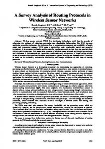
The selected path is then added to the already selected sensors at that stage. The algorithm terminates when the selected set of sensors completely cover the given query region. 3. Routing algorithms based on sensor position Routing in WSN is a key technology and very challenging problem. Many routing algorithms have been proposed to satisfy the requirement of sensor networks. Based on the position finding technology, routing algorithms attract more attention since position-based routing can decrease the complexity of routing and reduce the consumption. To position-based routing algorithms, it is required that (a) sensors can know its position according to suitable locating technology; (b) the sensing area is totally covered by sensors; (c) the connectivity is assured. In this paper, position information also includes relative position information, such as the hop-number distance. In this section, the position-based routing algorithms are surveyed and the different algorithms belonging to different categories are described in detail. Otherwise, the algorithms are also compared based on some metrics. 3.1 Flooding-based routing Flooding is classical and stateless mechanisms to relay data. In flooding, each sensor broadcasts receiving packets to all its neighbors. This process does not stop until the packet reaches the destination or the maximum hop number of the packet is reached. Although flooding is very easy to implement, it has several drawbacks, such as implosion, overlap and resource blindness [33]. In order to avoid the broadcast storm problem, different methods are proposed to limit the naïve flooding. Random flooding is one of improved flooding. In random flooding, sensors first receive a packet and then transmit the packet to all its neighbors with probability p. Other same packets are ignored. Based on random flooding idea, Braginsky David et al. [34] proposed rumor routing algorithm, which can be an alternative of naïve flooding. The basic idea of rumor routing can be described as follows: (1). When an event is occurred in a region of the network, sensing nodes create some event agents and propagate them along the network. Each node randomly forwards event agents to a neighbor, shown as Figure.3. (2). When event agent propagating the path to Event 2 comes across a path to Event 1, it begins to propagate the aggregate path to both, shown as Figure.4. (3). Each event agent has an event table containing the original event and every event visited in the trajectory. When an event agent meets a node, sensors’ event table is updated by the event agent, shown as Figure.5. (5). In order to join the path, the query agent is created and propagated along random path. Later queries can be routed along these agent-generated paths. It has been proved that the paths created by query and event agents have a very high possibility to intersect. The problem in rumor routing is that the forwarding of agent is random. So, it is possible that the paths of agents are too long. If the number of agents is large, the energy consumption is too much. Inspired by rumor routing, Tarun Banka et al. [35] proposed zonal rumor routing (ZRR) algorithm, in which rumor routing can be considered as a special case of ZRR when only one node belongs to one zone. ZRR enables the rumors to spread to a larger part of the network with high energy efficiency by partitioning the network into zones. ZRR can improve the percentage query delivery and requires fewer transmissions to reduce the total energy consumption in a sensor network.

Algorithms 2009, 2

164

Figure 3. Event agent [34].

Figure 4. Agents aggregate paths [34].

Figure 5. Agents optimize longer paths [34].

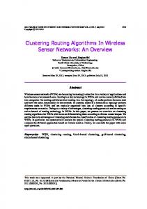
These rumor routing versions only use relative position information. Based on the precise position of its neighbors, Shokrzadeh et al. proposed directed rumor routing (DRR) [36, 37]. DRR propagates the event agents and the query agents in straight lines, instead of using purely random walk paths, centered at the source point and the sink point. In DRR, there is two phases for calibration. In the first phase, each node sends a Hello message containing its position to its neighbors and builds a list of its neighbors along with their positions. At the second phase each node detects if it is in the edge of the network in order to prevent the node from unnecessary traversing in the edges of the network. Firstly, each agent must carry the location of source. Then, at each step, the packet is forwarded to a neighbor with least deviation on the forward direction (Figure 6) using the location information of neighboring nodes. Otherwise, the packet is misrouted to a neighbor farthest from the source (Figure 7). In each step, a previously used node is not selected to route the packet to avoid cycles unless it is the only remaining node.

Algorithms 2009, 2 Figure 6. Routing in normal mode [36].

165 Figure 7. Routing in misroute mode [36].

Similar to DDR idea, many routing algorithms are proposed to limit flooding in a small area. Jaemin Son et al. proposed a limited flooding routing scheme for WSN [38]. The sink floods Sector Setup Packet (SSP) contains its location information and angular size. Each sensor receiving a SSP can decide its own sector (S, Figure.8) and track (T, Figure.9) and memorizes its sector and track numbers unless its energy is drained. The sink forms one-hop neighbor list consisting ID, a sector number, and the amount of remaining energy. The list is updated by an implicit ACK, which can locate a brokenlink during the RTT. When the sink needs information on a specific area, it disseminates a query including a sector number and track number to a specific sector and track. Each sensor receiving the query can decide its action. If the sector number included in the query is equal to that of the sensor node and if the track number contained in the query is higher than that of the sensor node, the sensor node forwards the received query to its neighbors. Otherwise, it discards the query. So, the flooding is limited in a specific area. If the link from the sink to sensors in the sector is broken, the sink selects one node with the largest energy as REPLY node, which floods the query received from the sink. Figure 8. Direction angle and sector number [38].

Figure 9. Track number [38].

Based on different idea to limit the flooding area, Zhang proposed several limited flooding algorithms [39, 40], which is inspired by the LAR (Location-Aided Routing) [41]. (1) In Figure.10, a rectangular limited flooding area can be constructed according to the position information of S

Algorithms 2009, 2

166

(source) and D (destination). The packets sent by S include the position information of left-bottom and right-top of the rectangle. If sensor receiving the packets is in the rectangle, it forward the packets to its neighbors. Otherwise, the packets are discarded. In Figure.10, r is a parameter to enlarge or reduce the flooding area. (2) In Figure.11, a flooding area is limited by the distance from S to D. The packets include the position information of S and D and it is very easy to calculate Dist-S (the distance from S to D). Each sensor can calculate Dist-X (the distance between the sensor, X, to D). If Dist-X is less than Dist-S, the packet is forwarded to other sensors. Otherwise, the packets are discarded. The parameter, Δ, is used to adjust the Dist-S. (3) In Figure.12, the angleSOM can be calculated based on RS, Rd and the position information of S and D. Receiving the packet, the sensor, X, can calculate the angleSOX. If angleSOX is less than angleSOM, the sensor forwards the packet. Otherwise, the packet is discarded. RS and Rd are the parameters and can adjust the size of flooding area. In this algorithm, the angle is fixed. (4) In Figure.13, receiving the packet with relative information, each sensor, X, π | XD | π )], } . |XD| and |SD| denote the distance from calculates the angleDXM based on min{ × [(1 + (1 − 4 | SD | 2 X and S to D separately. If the angleDXM calculated by X is larger than the angleDXM in the receiving packet, the packet is discarded. Otherwise, the packet is forwarded. Based on this algorithm, the area is reduced if the packet is more far from D. So, the flooding area is dynamic. Figure 10. Rectangular limited flooding area [39].

Figure 12. Static angle area [39].

Figure 11. Distance limited flooding area [39].

Figure 13. Dynamic angle area [39].

Algorithms 2009, 2

167

Flooding-based routing algorithms are easy to realize and maintaining the routing information is unnecessary. Table 1 compares random flooding, rumor routing and limited flooding according to different parameters. The results in the table are gotten by comparing the algorithms belonging to flooding-based routing. It is noted from the table that limited flooding is suitable to the applications in small area and rumor routing is suitable to the applications in large area. Table 1. Comparison among random flooding, rumor routing and limited flooding. Random flooding

Rumor Routing

Limited flooding

Energy consumption

Low

Middle

High

Negotiation-based

No

Yes

No

Complexity

Low

Low

Low

Reliability

No

Yes

Yes

Scalability

Middle

Good

Low

Multipath

No

Yes

Yes

3.2 Curve-based routing CBR (curve-based routing) is regarded as a hybrid technique combining source based routing [42] and Cartesian forwarding [43]. CBR is also similar to TBF (trajectory based forwarding) [44]. First, CBR is initiated by the source, which is similar to source based routing, but without specifying all the intermediate nodes. Second, in CBR, each sensor takes greedy action to forward the packet, which is similar to Cartesian forwarding, based on the distance to the predefined curve. The basic idea of CBR can be described as follows [45]: (1) a source node selects a suitable curve and encodes the curve into each packet; (2) upon receiving the packets, intermediate nodes decode the curve and use greedy strategies to decide next-hop to be forwarded and construct dynamic forwarding tables (DFT); (3) the sequent packets can be forwarded according to the constructed DFT; (4) after sending a number of packets, sources select another curve and forward packets along this curve. According to the basic CBR idea, the whole routing process can be described briefly as follows: The source (S) selects a suitable curve and encodes it into the packets. Then intermediate nodes select one node as next-hop in its neighbors according to greedy strategies and construct DFT. The sequent packets can be forwarded by lookup DFT. The intermediate nodes, such as P in Figure.14, will record the number of forwarded packets and tell its previous hop node (PH), such as M, to select another node, Q, to replace it. If M can’t find a suitable node according to the greedy strategy, it will send a special packet to inform S to select another curve to forward packets. After sending a number of packets along curve C1, S selects another curve, C2, to forward packets. These curves can be selected evenly in exploring area to balance the energy consumption of nodes effectively.

Algorithms 2009, 2 Figure 14. CBR model [45].

168 Figure 15. Next-hop selection [45].

In CBR model, there are two key problems: how to select the forwarding curve and how to select the next-hop. About the forwarding curve, although some simple curves, such as Beeline and Cosine, can be used in general applications, the curve parametric form is more suitable in order to avoid dangerous or doubtful area. Bezier curve is one of popular parametric curves [44, 46]. Compared with Bezier curve, B-spline curve has the following advantages [45]: (1) the computation cost is lower because the degree of the curve is independent on its control points; (2) a B-spline curve is naturally connected, so its shape can be controlled easily. The disadvantage of B-spline curve is that S and D are not the start point and end point of curve based on the original equation of B-spline curve. In [45], in order to make the B-spline curve start from S and end to D, Equation.1 is changed as following: (1) Let t=0 and t=1 respectively to get Equation.2. (2). Set P0,2(0)=S and P0,2 (1)=D, then select one control point V1, the other two control points can be calculated. The three control points (V0, V1, V2) can ensure that S and D are the start and end points of the B-spline curves respectively. The coordinates of control points and t are encoded and forwarded. Receiving the packet, the intermediate sensors can calculate and judge itself on the curve or not based on the greedy next-hop selection strategy.

(1)

t =0 t =1

P0,2 (0) = ( V0 + V1 )/ 2⎫⎪ ⎧⎪V0 = 2P0,2 (0) − V1 ⎬ ⇒⎨ P0,2 (1) = ( V1 + V2 )/ 2 ⎪⎭ ⎪⎩V2 = 2P0,2 (1) − V1

(2)

How to select next-hop is another important issue in CBR. Basically, the next-hop node should make sure that the packet advances along the trajectory curve, not backwards. Depending on application and user criteria, different selecting strategies have been proposed [46] (Figure.15): (1) Random: select the next node randomly from the neighborhood. (2) Closest to Curve (CTC): select the node closest to the curve from its neighbor. (3) Least Advancement on Curve (LAC): forward to the node closest to the current node. (4) Most Advancement on Curve (MAC): forward the packets to the farthest node along the curve. (5) Lowest Deviation from Curve (LDC): the best next node Ni should be selected such that the line between N0 and Ni must have the smallest deviation from the trajectory

Algorithms 2009, 2

169

compared to the other lines between N0 and any other node in N0’s neighborhood. In Figure.15, Ni (i=1…4) is the candidate of N0’s next-hop. N3, N2, N1 and N4 are selected as the next-hop based on CTC, LAC, MAC and LDC separately. Figure 16. Applications of CBR [44].

CBR is a simple and effective routing strategy for sensor network. Many applications can benefit from CBR framework. Figure.16 shows some applications of CBR [44]. (1) Broadcast: use a number of radial outgoing lines that are reasonably close to each other, shown as Figure.16(a). It can achieve a similar effect without all the communication overhead involved by receiving duplicates in classical flooding. A simple five-step discovery scheme (Figure.16(d)) based on linear trajectories may be used to replace traditional broadcast based-discovery. (2) Multi-path: both disjoint (Figure.16(b)) and braided (Figure.16(c)) paths are useful in providing resilience. It’s easy to construct multi-path according to different control points [47]. (3) Coverage: a source would indicate the directions and the lengths of the lines that would achieve a satisfactory coverage (Figure.16(e)). (4) Multicast: If unicast communication is modeled by a simple curve, multicast is modeled by a tree in which each portion might be a curve, or a simple line. Distribution trees are used for either broadcasting (Figure.16(e)), or multicast routing (Figure.16(f)). 3.3 Grid-based routing Grid-based routing algorithms use grid as the basic routing infrastructure. Considering different characteristics of networks, different grid construction methods have been proposed. In [48], grid location service (GLS) is proposed for Ad Hoc routing where the nodes are totally mobile. In [49], two-tier data dissemination (TTDD) grid is constructed for large-scale WSN where multiple sinks are mobile. In [50, 51], a virtual grid (VG) is constructed for routing in WSN where all sensors are static. In grid-based routing algorithms, how to construct and maintain the grid is the key problem.

Algorithms 2009, 2

170 Figure 17. Global partitioning of the area [48].

Figure 18. The location server of B in different order [48].

GLS is based on the idea that a node maintains its current location information in some location servers distributed throughout the network [48]. GLS provides for distributed location lookups by replicating the knowledge of a node’s current location at a small subset of the network’s node, which is referred to as the node’s location servers. In GLS, grid-based partition is arbitrary and any other balanced hierarchical partition of the space can be used. It is presumed that all nodes know the same global partitioning of the area into a hierarchy of grids with squares of increasing size, as shown in Figure.17. One smallest square is called an order-1 square. Generally, four order-1 squares make up an order-2 square, and so on. Sometimes, a particular order-n square is part of only one order-n+1 square in order to avoid overlap. This maintains an important invariant: a node is located in exactly one square of each size. If square size is increased, fewer location servers are selected for nodes at greater distances. The location servers are not specially designated and are acted by each node. The location servers for a node are relatively dense near the node but sparse farther from node to balance the efficiency and energy consumption. Each node recruits nodes with IDs “close” to its own ID to serve as its location

Algorithms 2009, 2

171

servers. The node closest to node, X, in ID space is defined to be the node with the least ID greater than X. A node selects location servers in each sibling of a square that contains the node, as shown in Figure.18. In Figure.18, B recruits three servers in order-1 squares (28, 2 and 63), three servers in order-2 squares (26, 31 and 43), and three servers in order-3 squares (37, 19 and 20). Once all nodes have provided their coordinates to their location servers, the grid state is complete. If one node (S) sends the data to the destination (D), S sends the query to the least node greater than or equal to D for which S has location information. The query is forwarded in the same way. Eventually, the query will reach a location server of D, which will forward the query to D. Since the query contains S’s location, D can respond directly using geographic forwarding. Although GLS is effective to query and forward data in Ad Hoc, the construction and maintenance of grid is too complicated and not energy-aware to apply to WSN. Sink mobility also brings new challenges to large-scale WSN because the location information of mobile sink's should be continuously updated through the sensor field, such as Directed Diffusion [52] and GRAB [53]. It causes the excessive drain of sensor’s limited energy and increases the collisions in wireless link. Ye Fan et al. proposed the two-tier data dissemination (TTDD) idea to resolve this problem [49]. There are two tiers: the lower tier is within the local grid square of the sink's current location (called cells), and the higher tier is made of the sensors closest to grid points (called dissemination nodes). Each data source proactively builds a grid structure which enables mobile sinks to continuously receive data on the move by flooding queries within a local cell. In TTDD, the grid is constructed by sources. A source divides the plane into a grid of cells. Each cell is an α*α square. A source itself is at one crossing point of the grid and propagates the parameters (α) in the whole field. The other dissemination points can be calculated based on the simple equation: {xi=x+i*α; yi=y+j*α; i,j=…,-3, -2, -1, 0, 1, 2, 3,…}. The source sends a data-announcement message to its four dissemination points (Lp) and the neighbor node continues forwarding the data announcement message in a similar way till the message stops at a node that is closer to Lp than all its neighbors. If this node's distance to Lp is less than a threshold α/2, it becomes a dissemination node serving Lp for the source. The data announcement message is recursively propagated through the whole sensor field so that each dissemination point on the grid is served by a dissemination node. Figure.19 shows a grid constructed by a source B. It should be pointed out that the crossing points of two blue lines are virtual and the black nodes around crossing points are the dissemination nodes. Another key problem is how to maintain the grid structure. TTDD uses the Grid Lifetime to control the maintaining time. The data announcement message includes Grid Lifetime. So, Grid Lifetime is known by the dissemination nodes when the grid is built. If the lifetime elapses and the dissemination nodes do not receive any further data announcements to update the lifetime, they clear their states and the grid no longer exists. Proper grid lifetime values depend on the data availability period and the mission of the sensor network.

Algorithms 2009, 2 Figure 19. The grid constructed by B [49].

172 Figure 20. Query and data forwarding [49].

After the grid is constructed, the whole data forwarding process can be described as follows. The sink floods its query within a cell and only sensors located at grid points need to acquire the forwarding information. When the nearest dissemination node for the requested data receives the query, it forwards the query to its upstream dissemination node toward the source, which in turns further forwards the query, until it reaches either the source or a dissemination node that is already receiving data from the source. This query forwarding process lays information of the path to the sink, to enable data from the source to traverse the same two tiers as the query but in the reverse order. Combining the grid structure and curve-based routing idea, Zhang et al. proposed the grid-based routing algorithms (GBRA) [50, 51]. The algorithm is used to the static WSN, where the source and sink are fixed. The algorithms can be divided into several stages: the local topology built stage (LTBS), grid built stage (GBS), path constructed stage (PCS), density controlled stage (DCS) and data forwarded stage (DFS). Figure 21. The constructed grid by sink [50].

Figure 22. Single grid with path [50].

In LTBS, the main purpose of this stage is to build a neighbor table (NT) through finding the direct neighbors of each node. Once node is scattered, the node will send topology finding packets (TFP) three times during a certain period. In GBS, the aim is to divide the network into grid with suitable size similar to TTDD and let each node know which grid it belongs to, shown as Figure.21. Meanwhile,

Algorithms 2009, 2

173

relational information (location and data type needed) about sink is distributed. In Figure.21, (x, y) is a theoretic point and the service node (SN) of (x, y) is selected. For each vertex, two SN are selected. SN only deals with those packets coming from the same grid and ignores those coming from neighbor grid. In PCS, the aim of this stage is to construct a path across one single grid from one SN to another SN based on curve routing algorithm, which is described in [45]. Based on CBGR, two theoretic vertexes and a randomly node are selected as control points in PCS. Because two vertexes are neighbor, one vertex can induce the other vertex. In DCS, the aim is to make redundant nodes sleep, shown as Figure.22. In Figure.22, the black nodes are working and the gray nodes are sleeping. The node on the path (named Initiating Node, IN) is working node. IN chooses other working nodes by WNSP (Working Nodes Selected Packets) as follows: (1) Supposing the coordinates of IN, N, is (XN,YN), N chooses nodes whose abscissa are between (XN－Δ) and (XN＋Δ) from next-hop table (NT); (2) N chooses the node which has maximum |Y-YN| as working node from NT, constructs WNSP and sends out; (3) Receiving the WNSP, only the node whose ID is included in the WNSP will deal with WNSP; (4) The procedure completes until to find a node near the other edge in the grid as shown in Figure.22: N->M->O->P->Q, and N->R, where Δ is variable and can be adjusted according to the number of IN on the curve. Similar to the basic grid idea, there are other algorithms with different routing graph. GPSR (Greedy Perimeter Stateless Routing) is geographic routing based on greedy strategy, which finds neighbors closer to the destination and forwards the packet to the neighbor closest to the destination [54]. GPSR uses Right-Hand Rule to traverse the edges of a void. GPSR picks the next anticlockwise edge. Shown as Figure.23, x receives a packet from y, and forwards it to its first neighbor counterclockwise about itself, z. Finally, the routing path forms the polygon, shown as Figure.24. In Figure.24, D is the destination and x is the node where the packet enters perimeter mode. Solid arrows denote the forwarding hops. Figure 23. Right-hand rule [54].

Figure 24. Forwarding path based on GPSR [54].

Grid-based routing algorithms are similar to hierachical routing strategy. The structure of grid provides some advantages to design the effective routing algorithms. Table 2 compares GLS, TTDD and GBRA according to different metrics. The results in the table are gotten by comparing the algorithms belonging to grid-based routing. It is noted that grid-based routing algorithms is suitable to deal with the mobility problem.

Algorithms 2009, 2

174 Table 2. Comparison among GLS, TTDD and GBRA. GLS

TTDD

GBRA

Energy consumption

High

Middle

Low

Negotiation-based

No

Yes

Yes

Complexity

High

Middle

Low

Reliability

High

Middle

Middle

Scalability

Low

Good

Middle

Mobility

All moving

Sink moving

No

3.4 Ant algorithm-based intelligent routing Compared with the previous position-based routing algorithms, ant algorithm-based intelligent routing algorithms are complicated. It is found that the ants have the ability of finding the best route between ant’s cave and food via detecting the pheromone [55], which is the original idea to design ant algorithm. In travel, the shorter the path is, the higher the pheromone concentration is, so ants can find right field in searching space using positive feedback mechanism. As social insects, ants can show a colony intelligent behavior via cooperation while carrying out some tasks that can’t be finished by the individual. Ant algorithms are used to solve not only the TSP problem, but also the anycast routing and query processing problems and so on [56, 57]. Combined with the idea of ant algorithm and position information, ant algorithm-based intelligent routing algorithms have been proposed successively for WSN [58, 59]. In order to set up the routing, each source node sends several detection packets (ants) to the sink node. Each ant packet has the following information: the visited list, the edge list and the position of the sink. The visited list is used to record the nodes, which have been passed by ants, and the initial value of it is empty. The edge list is used to record the edges ant selected when detecting. Each node maintains a table including the position information of their neighbor nodes, which can be updated by hello messages between neighbor nodes periodically. Each of the source nodes can obtain the position information of the sink by receiving the interests the sink flooded and generate the ants. Figure 25. The illustration of the deflexion angle.

Before the ant-based intelligent algorithm is described, some parameters are explained firstly. In Figure.25, node u is one of the neighbors of node v. θ is denoted as the deflexion angle of the edge e at node u relative to the sink. The number of the source nodes is m. The detailed steps are described as follows:

Algorithms 2009, 2

175

Step.1: The pheromone value of each edge of the network is initialized to 1. There are m ants in the m source nodes respectively (The source node k sends the ant k and k ∈ [1, m] ). And the source node k is inserted into the visited list of ant k. Step.2: Assume that the node at which ant k currently arrived is v, and the set Ωv contains all the neighbor nodes of the node v, the local rules for each ant are as follows: 1) If node v is the sink node, the destination is found and the ant stops detecting. 2) Else, judge each of the neighbor nodes u ∈ Ωv of node v to find out whether they are in the visited list of ant k or not. Set the number of the neighbors of node v that is not in the visited list of ant k is R. then, a) If R>0, continue to detect each of the R available neighbor nodes. If the current detected node ut is the sink node, then set it as the next step node. Otherwise, follow the rules below: ‹ Based on the coordinates of node v, node ut and the sink node, calculate the cosine value of angle θ < v ,u > by the formula of cosines. Then calculate the diverted weight of t

the node ut : ρ< v ,u > = [ Phere



t

] ⋅ cos θ e t

, where the Phere



is the pheromone value of

the edge e< v ,u > ; t

‹ Select the neighbor node which holds the largest diverted value ρ< v ,u > as the next hop t

node. If condition Phere



there

are

several

= max{Phere , Phere ," , 2

1

Phere

nodes satisfied the } , choose the node which owned

the longest edge e< v ,u > ( t ∈ [1, R] ) as the next hop node. t

b) If R=0, that is, all the neighbors of node v are in the visited list of ant k. The ant k should come back to the previous node. of the selected edge e< v ,u > of the network as 3) The ant k assigns the pheromone value Phere

t

2 ⋅ Phere . t

Step.3: For each ant k ( k ∈ m ), the next hop node and the corresponding edge should be inserted into its visited list and edge list separately. Then judge whether all the visited lists contain the sink node. If yes, the algorithm goes into the end. Otherwise, for each ant k, set the next hop node as the current node, go to Step 2. Although ant algorithm-based routing algorithms is a little complicated to realize, the algorithm has good performances to find optimum paths and collecting data to the sink by positive feedback. It has the potential to resolve the different problems, such as data broadcasting [60] and data gathering [61], in WSN. 3.5 Performance comparison In this article, these routing algorithms based on position information are reviewed and classified into four categories: flooding-based, curve-based, grid-based and ant algorithm-based. Though these algorithms have the same assumption, each category still has its unique characteristics. In Table 3, the characteristics are summarized and compared according to some popular metrics [4]. The results are gotten based on the general routing algorithms of different categories.

Algorithms 2009, 2

176

Table 3. Comparison among four kinds of position-based routing algorithms. Flood-based

Curve-based

Grid-based

Ant algorithm-based

Energy consumption

High

Low

Low

Middle

Negotiation-based

No

No

Yes

Yes

Complexity

Low

Low

Middle

High

Reliability

High

Middle

Middle

Middle

Scalability

Low

Good

Good

Middle

Multipath

Yes

Yes

No

Possible

Data aggregation

No

No

Possible

No

Query-based

No

No

No

Yes

Though position-based routing algorithms have some obvious advantages, there are several problems. First, how to realize data aggregation is difficult because position-based routing algorithms are flat routing and there are not clusters to aggregate data. In sensor networks with dense deployed nodes, one phenomenon can be found by many nodes near the phenomenon. If each sensor detecting the same phenomenon sends the data alone, it is unnecessary and consumes too much energy. So, data aggregation is important to extend the application areas of position-based routing algorithms. Second, how to improve the reliability of position-based routing is another problem. Most position-based routing algorithms are stateless. It is hard to judge that the next-hop has forwarded the data correctly or not. Considering that the sensor is low cost and tends to fail, the problem is more serious. Otherwise, position-based routing algorithms with the characteristics of QoS, security or multipath are necessary to special applications. These can also be regarded as the future directions and are discussed in detail in section 4. 4. Conclusion and Open Issues WSN has many unique characteristics, different from traditional networks. It also introduced much challenges to design suitable routing algorithms, which has attracted a lot of attention in the recent years. Different from the survey on routing algorithms, we have summarized recent research results on position-based routing in WSN. It is classified into four main categories: flooding-based, curve-based, grid-based, and ant-based intelligent. Their performance is also compared based on some popular metrics. Though all these algorithms are based on the position information of sensors, how to use the position information is different. In flooding-based routing, the position information is used to limit the flooding area by constructing different flooding area. Compared with other algorithms, floodingbased routing algorithms are very easy to realize. Curve-based routing algorithm is one kind of novel routing strategy. Position information is used to construct the routing curve and forward the data. Curve-based routing combine source based routing with Cartesian forwarding. The source initiates the algorithms, selects the forwarding curve and encodes the parameter, but without specifying all the intermediate nodes. Each sensor takes greedy action to forward the packet based on local information.

Algorithms 2009, 2

177

Gird-based routing algorithms are based on the grid structure. The key problem is how to use the position information to construct and maintain the grid. In different algorithms, the grid is constructed by different sensors (for example, source, sink). Once the grid is constructed, data forwarding can use suitable methods, such as geographical greedy forwarding, curve-based forwarding. Ant-based intelligent routing algorithm is originated from the phenomena that ants always find the optimal path when finding food. The algorithms are similar to the ant’s colony intelligent behavior via cooperation. Through several ants to the sink, the algorithms can automatically form the optimal path based on the position information. Although extensive efforts have been exerted so far on the position-based routing problem in WSN, there are still many challenges because of the unique characteristics of WSN. Future trends in routing focus on different directions and all share the common objective of prolonging network lifetime, handling the overhead of mobility and topology changes in an energy-constrained environment. In the last section, some of these directions related with position information are summarized as follows: (1) The redundancy detection mechanism. In WSN, node is typically dense deployment. It is unnecessary that all these sensors simultaneously work. How to control the number of working sensors is valuable. Especially, the strategy combining the coverage algorithms with routing technology is hopeful. Another interesting idea is exploiting effective sensordensity control algorithms. (2) The secure routing problem. Security is very difficult to assure because the unsymmetrical encryption strategy is unsuitable for the energy requirement. Only the symmetrical encryption strategy can be used, which also make key assignment and time synchronization difficult. Most of current routing algorithms aim to optimize the energy consumption. Though there are some security strategies for routing, more attention still needs to be paid to satisfy the application requirement, such as battlefield environment. (3) QoS routing problem. To the video and imaging sensors and real-time applications, QoS routing in WSN should ensure suitable bandwidth (or delay) through the duration of connection as well as providing the use of most energy efficient path. Currently, there is very little research on routing strategy with QoS requirements in resource constrained environment, which is also a challenge task. (4) Intelligent routing mechanism. In WSN, most effort aims to design simple routing strategy, which is easy to realize and energy-aware. Considering those complicated application requirements, the intelligent routing technology is suitable when the sensors have more usable resources. Combining with position information, it’s hopeful to design the energyaware intelligent routing. (5) Node mobility problem. Most of the current protocols assume that the sensor nodes are stationary. However, the moving sink or sensors can not be avoided in some special applications, which make nodes’ position change frequently. If the node position is updated frequently or not is a problem. New position-based routing ideas are needed in order to balance the topology update and the energy consumption. (6) Data fusion strategy. As an energy-aware operation, data fusion or aggregation is important and popular in hierarchical routing. Though most position-based routing

Algorithms 2009, 2

178

algorithms are flat routing, it seems that data fusion is hard to use. Considering the gridbased routing algorithms, there are natural clusters making data fusion. How to realize data fusion in one grid is also an interesting problem to explore. Other possible future research for routing protocols also includes achieving global behavior with localized algorithms, routing technology with data compression, etc. Most of these issues can be considered with position information. Acknowledgements Part of this work was supported by Science and Technology Plan Items of Hunan Province (No. 2008GK3089) and China's Post-doctoral Science Foundation (No. 20080441260). References 1. 2. 3. 4. 5. 6.

7. 8. 9.

10. 11. 12.

Akyildiz, I.F.; Su, W.; Sankarasubramaniam, Y.; Cayirci, E. Wireless sensor networks: a survey. Computer Networks 2002, 38 (4), 393–422. Kahn, J. M.; Katz, R.H.; Pister, K.S.J. Next century challenges: mobile networking for smart dust. In Proceedings of ACM MobiCom, Seattle, 1999, pp. 271-278. Xiao, Renyi; Wu, Guozheng. A survey on routing in wireless sensor networks. Progress in natural science 2007, 17(3), 261-269. Jamal, N. Al-Laraki; Ahmed, E. Kamal. Routing techniques in wireless sensor networks: a survey. IEEE wireless communication 2004, 11(6), 6- 28. Stojmenovic, I. Handbook of sensor networks: algorithms and architectures. John Wiley & Sons: New York, NY, USA, 2005. Delin, L.A.; Jackson, S.P.; Johnson, D.W.; Burleigh, S.C.; Woodrow, R.R.; McAuley, M.; Britton, J.T.; Dohm, J.M.; Ferré, T.P.A.; Felipe, I.; Rucker, D.F.; Baker, V.R. Sensor web for spatiotemporal monitoring of a hydrological environment. In Proceedings of Lunar and Planetary Science Conference, League City, 2004, pp. 1430-1438. Hill, J.; Szewczyk, R.; Woo, A. System architecture directions for networked sensors. In Proceedings of ASPLOS-IX, Cambridge, 2000, pp. 1-18. Perrig, A.; Szewczyk, R.; Tygar, J.D. SPINS: Security Protocols for Sensor Networks. Wireless Networks 2002, 8, 521-534. Corke, P.; Hrabar, S.; Peterson, R.; Rus, D.; Saripalli, S.; Sukhatme, G. Autonomous deployment and repair of a sensor network using an unmanned aerial vehicle. In Proceedings of IEEE International Conference on Robotics and Automation, Kenmore, 2004, pp. 3602-3608. Callaway, E.H. Wireless Sensor Networks: Architectures and Protocols. CRC Press: Boca Raton, FL, USA, 2004. Akkaya, K.; Younis, M. A survey on routing protocols for wireless sensor networks. Ad Hoc Networks 2005, 3, 325–349. Langendoen, K.; Reijers, N. Distributed localization in wireless sensor networks: a quantitative comparison. Computer Networks 2003, 43 (4), 499 – 518.

Algorithms 2009, 2

179

13. Mao, G.; Barıs¸ F.; Anderson, B.D.O. Wireless sensor network localization techniques. Computer Networks 2007, 51(10), 2529-2553. 14. Koks, D. Numerical calculations for passive geolocation scenarios. Tech. Rep. DSTO-RR-0000, 2005. 15. Rappaport, T.; Reed, J.; Woerner B. Position location using wireless communications on highways of the future. IEEE Communications Magazine 1996, 34(10), 33–41. 16. Niculescu, D.; Nath, B. Ad hoc positioning system (APS) using AoA. In Proceedings of INFOCOM, San Francisco, 2003, pp. 1734–1743. 17. Schmidt, R. Multiple emitter location and signal parameter estimation. IEEE Transactions on Antennas and Propagation 1986, 34(3), 276–280. 18. Roy, R.; Kailath, T. ESPRIT-estimation of signal parameters via rotational invariance techniques. IEEE Transactions on Acoustics, Speech, and Signal Processing 1989, 37(7), 984–995. 19. Priyantha, N.; Chakraborty, A.; Balakrishnan, H. The cricket location-support system. In Proceedings of the Sixth Annual ACM International Conference on Mobile Computing and Networking (MOBICOM), Boston, 2000, pp. 32–43. 20. Savvides, A.; Han, C.-C.; Strivastava, M. B. Dynamic fine-grained localization in ad-hoc networks of sensors. In Proceedings of the 7th annual international conference on Mobile computing and networking (MobiCom), Rome, 2001, pp. 166–179. 21. Prasithsangaree, P.; Krishnamurthy, P.; Chrysanthis, P. On indoor position location with wireless LANs. In Proceedings of 13th IEEE International Symposium on Personal, Indoor and Mobile Radio Communications, Lisbon, 2002, pp. 720–724. 22. Bahl, P.; Padmanabhan, V. RADAR: an in-building RF-based user location and tracking system. In Proceedings of IEEE INFOCOM, Tel-Aviv, 2000, pp. 775–784. 23. He, T.; Huang, C.; Blum, B. M.; Stankovic, J. A.; Abdelzaher, T. Range-free localization schemes for large scale sensor networks. In Proceedings of the 9th annual international conference on Mobile computing and networking (MobiCom), San Diego, 2003, pp. 81–95. 24. Nagpal, R.; Shrobe, H.; Bachrach, J. Organizing a global coordinate system from local information on an ad hoc sensor network. In Proceedings of Second International Workshop on Information Processing in Sensor Networks (IPSN), Palo Alto, 2003, pp. 333–348. 25. Niculescu, D.; Nath, B. Ad hoc positioning system (APS). In Proceedings of GLOBECOM, San Antonio, 2001, pp. 2926–293. 26. Masoomeh, Rudafshani; Suprakash, Datta. Localization in wireless sensor networks. In Proceedings of the 6th International Conference on Information Processing in Sensor Networks, Cambridge,USA, 2007, pp. 51-60. 27. Wu, J.; Li, H. A dominating-set-based routing scheme in ad hoc wireless networks. Telecommunication Systems Journal 2001, 18, 13-36. 28. Alzoubi, K. M.; Wan, P.-J.; Frieder, O. Message-optimal connected dominating sets in mobile ad hoc networks. In Proceedings of the International Symposium on Mobile Ad Hoc Networking and Computing (MobiHoc), Lausanne, Switzerland, 2002, pp. 157-164.

Algorithms 2009, 2

180

29. Slijepcevic, S.; Potkonjak, M. Power efficient organization of wireless sensor networks. In Proceedings of the International Conference on Communications (ICC), Helsinki, Finland, 2001, pp. 472-476. 30. Lin, F.Y.S.; Chiu. P. L. A near-optimal sensor placement algorithm to achieve complete coverage/discrimination in sensor networks. IEEE Communications Letters 2005, 9(1), 43-45. 31. Tian, D; Georganas, N.D. A node scheduling scheme for energy conservation in large wireless sensor networks. Wireless Communications and Mobile Computing 2003, 3(2), 271-290. 32. Gupta, H; Das, S.R.; Gu, Q. Connected sensor cover: Self-Organization of sensor networks for efficient query execution. In Proceedings of the ACM International Symposium on Mobile Ad Hoc Networking and Computing(MobiHOC), Annapolis, USA, 2003, pp. 189-200. 33. Heinzelman, W.; Kulik, J.; Balakrishnan, H. Adaptive protocols for information dissemination in wireless sensor networks. In Proceedings of the 5th Annual ACM/IEEE International Conference on Mobile Computing and Networking (MobiCom), Seattle, USA, 1999, pp. 174-185. 34. Braginsky, D.; Estrin, D. Rumor routing algorithm for sensor networks. In Proceedings of the 1st ACM international workshop on wireless sensor networks and applications, Atlanta, USA, 2002, pp. 22-31. 35. Banka, T.; Tandon, G.; Jayasumana, A.P. Zonal rumor routing for wireless sensor networks. In Proceedings of International Conference on Information Technology, Coding and Computing, Las Vegas, USA, 2005, pp. 562- 567. 36. Shokrzadeh, H.; Haghighat, A. T. Directed Rumor Routing in Wireless Sensor Networks. In Proceedings of ICEE, Iran, 2007. 37. Shokrzadeh, H.; Haghighat, A. T.; Tashtarian, F.; Nayebi, A. Directional Rumor Routing in Wireless Sensor Networks. In Proceedings of 3rd IEEE/IFIP International Conference in Central Asia on Internet, Tashkent, Uzbekistan, 2007, pp. 1-5. 38. Son, J.; Ha, N.; Kim, K.; Ryu, J.; Son, J.; Han, K. A Limited Flooding Scheme for Query Delivery in Wireless Sensor Networks. In Proceedings of International Workshop on Sensor Networks, volume 3842 of Lecture Notes in Computer Science, Harbin, China, 2006, pp. 276-280. 39. Zhang, J. On Routing Algorithms Based on Position Information for Sensor Networks. Master dissertation, Changsha: Hunan University, 2004. (In Chinese) 40. Zhang, J.; Lin, Y. P. An Angle-Area-Based Flood Routing Algorithm for Sensor Networks. Computer Engineering & Science 2005, 27(9), 59-61. (In Chinese) 41. Ko, Y. B.; Vaidya, N. H. Location-Aided Routing (LAR) in mobile ad hoc networks. Wireless Networks 2000, 6, 307–321. 42. Johnson, D. B.; Maltz, D. A. Dynamic source routing in ad hoc wireless networks. Mobile Computing 1996, 353, 153-181. 43. Finn, G. Routing and addressing problems in large metropolitan-scale internetworks. Technical Report ISI Research Report ISI/RR-87-180, University of Southern California, March 1987. 44. Niculescu, D.; Nath, B. Trajectory based forwarding and its applications. In Proceedings of 9th Annual International Conference on Mobile Computing and Networking, San Diego, USA, 2003, pp. 260 – 272.

Algorithms 2009, 2

181

45. Zhang, J.; Lin, Y. P.; Lin, M.; Li, P.; Zhou, S. W. Curve-Based Greedy Routing Algorithm for Sensor Networks. In Proceedings of International Conference on Computer Network and Mobile Computing, Lecture Notes in Computer Science, Zhangjiajie, China, 2005, vol. 2619, pp. 1125 – 1133. 46. Yuksel, M.; Pradhan, R.; Kalyanaraman, S. An Implementation Framework for Trajectory-Based Routing in Ad Hoc Networks. In Proceedings of IEEE International Conference on Communications’ 04, Paris, France, 2004, pp. 4062-4066. 47. Cheng, F. H.; Zhang, J. A Reliable Routing Algorithm for Sensor Network Based on Multi-path. In Proceedings of 9th International Conference on Control, Automation, Robotics and Vision, Singapore, 2006, pp. 1-3. 48. Li, J. Y.; Jannotti, J.; De, D. S. J.; David, C.; Karger, R.; Morris, R. A Scalable Location Service for Geographic Ad Hoc Routing. In Proceedings of the 6th ACM International Conference on Mobile computing and Networking (MobiCom'00), Boston, USA, 2000, pp. 120-130. 49. Luo, H. Y.; Ye, F.; Cheng, J.; Lu, S. W.; Zhang, L. X. TTDD: Two-Tier Data Dissemination in Large-Scale Wireless Sensor Networks. Wireless Networks 2005, 11, 161–175. 50. Zhang, J.; Li, G. A Density-Based Energy-Effective Routing for Sensor Networks. In Proceedings of the 6th World Congress on Control and Automation, Chongqing, China, 2006, pp. 3801-3804. 51. Peng, T. G.; Zhang, J. Grid-Based Routing Algorithm for Sensor Networks. In Proceedings of International Conference on Wireless Communications, Networking and Mobile Computing, Shanghai, China, 2007, pp. 2242-2245. 52. Intanagonwiwat, C.; Govindan, R.; Estrin, D. Directed Diffusion: A Scalable and Robust Communication Paradigm for Sensor Networks. In Proceedings of ACM International Conference on Mobile Computing and Networking (MobiCom), Boston, USA, 2000, pp. 56-67. 53. Ye, F.; Zhong, G.; Lu, S.; Zhang, L. GRAdient broadcast: a robust data delivery protocol for large scale sensor networks. Wireless Networks 2005, 11(3), 285-298. 54. Karp, B.; Kung, H. T. GPSR: Greedy perimeter stateless routing for wireless networks. In Proceedings of the Sixth Annual ACM/IEEE International Conference on Mobile Computing and Networking (MobiCom), Boston, USA, 2000, pp. 243–254. 55. Dorigo, M.; Gambardella, L.M. Ant colonies for the traveling salesman problem. BioSystems 1997, 43(2), 73-81. 56. Yu, J.P.; Lin, Y.P.; Lin, M.; Yi, Y.Q. Multi-constrained anycast routing based on ant algorithm. Chinese Journal of Electronics (CJE) 2006, 15 (1), 133-137. 57. Yu, J.P.; Lin. Y.P.; Zheng, J.H. Ant-based query processing for replicated events in wireless sensor networks. In Proc of the 2008 IEEE World Congress on Computational Intelligence (IEEE WCCI 2008), Hongkong, China, 2008, pp. 138-145. 58. Dorigo, M.; Birattari, M.; Stützle, T. Ant colony optimization-Artificial ants as a computational intelligence technique. IEEE Computational Intelligence Magazine 2006, 1(4), 28–39. 59. Li, W.; Lin, Y.P.; Tong, T.S.; Chen, Y.; Yu, J.P. A distributed data-centric routing algorithm based on ant algorithm for sensor networks. Mini-Micro Systems 2005, 26(5), 788-792. (In Chinese)

Algorithms 2009, 2

182

60. Li, S.; Yang, C.; Kang, J. An ant algorithm for data broadcasting and gathering in the sensor network. Jounal of Wuhan University (Natural Science Edition) 2006, 52(1), 100-104. (In Chinese) 61. Liao, W. H.; Kao, Y. C.; Fan, C. M. Data aggregation in wireless sensor networks using ant colony algorithm. Journal of Network and Computer Applications 2008, 31(4), 387-401.

© 2009 by the authors; licensee Molecular Diversity Preservation International, Basel, Switzerland. This article is an open-access article distributed under the terms and conditions of the Creative Commons Attribution license (http://creativecommons.org/licenses/by/3.0/).