A Systematic Cross-Comparison of Sequence Classifiers Binyamin Rozenfeld, Ronen Feldman, Moshe Fresko Bar-Ilan University, Computer Science Department, Israel
[email protected],
[email protected],
[email protected], Abstract In the CoNLL 2003 NER shared task, more than two thirds of the submitted systems used a feature-rich representation of the task. Most of them used the maximum entropy principle to combine the features together. Others used large margin linear classifiers, such as SVM and RRM. In this paper, we compare several common classifiers under exactly the same conditions, demonstrating that the ranking of systems in the shared task is due to feature selection and other causes and not due to inherent qualities of the algorithms, which should be ranked otherwise. We demonstrate that whole-sequence models generally outperform local models, and that large margin classifiers generally outperform maximum entropy-based classifiers.
1 Introduction Recently, feature-rich classifiers became state-of-the-art in sequence labeling tasks, such as NP chunking, PoS tagging, and Named Entity Recognition. Such classifiers are able to use any property of tokens and their contexts, if the property can be represented in the form of realvalued (usually binary) feature functions. Since almost all local properties can be represented in such a way, this ability is very powerful. Maximum-entropy-based models are currently the most prevalent type of feature-rich classifiers in sequence labeling tasks. Such models define a probability distribution over the set of labelings of a sentence, given the sentence. In this, such classifiers differ from the generative probabilistic classifiers, such as HMM-based Nymble (Bikel et al., 1999) and SCFG-based TEG (Rosenfeld et al., 2004), which model the joint probability of sequences and their labelings, and which can use only a very limited range of context features. An alternative feature-rich approach is discriminative models, trained by maximizing the margin between correct and incorrect labelings. Recently, the maximal margin classifiers were adopted for multi-label classifi-
cation (Crammer, Singer, 2001) tasks and for structured classification tasks (Taskar, Guestrin, and Koller, 2003). Another important difference among methods is their scope. The most often used methods are local, in the sense of modeling classification decisions separately for each sentence position. More recent methods model labeling of whole sequences. In this work we compare the performance of four different classifiers within the same platform, using exactly the same set of features. MEMM (McCallum, Dayne Freitag, and Pereira, 2000; Chieu and Ng, 2002) and CRF (Lafferty, McCallum, and Pereira, 2001; McCallum and Li, 2003) are a local and a wholesequence maximum entropy based classifiers. RRM (regularized Winnow) (Zhang and Johnson, 2003) and MIRA (McDonald, Crammer and Pereira, 2004) are a local and a whole-sequence maximal margin classifiers. We test the effects of different training sizes, different choice of parameters, and different feature sets upon the algorithms' performance. Our experiments indicate that whole-sequence models outperform local models, as expected. Also, although the effect is less pronounced, maximal margin models generally outperform maximum entropy based models. We will present our experiments and their results.
2 Experimental Setup The goal of this work is to compare the four sequence labeling algorithms in several different dimensions: absolute performance, dependence upon the corpus, dependence upon the training set size and the feature set, and dependence upon the hyperparameters.
2.1
Datasets
For our experiments we used four datasets: CoNLL-E, the English CoNLL 2003 shared task dataset, CoNLLD, the German CoNLL 2003 shared task dataset, the MUC-7 dataset (Chinchor, 1998), and the proprietary CLF dataset (Rosenfeld et al., 2004). For the experiments with smaller training sizes, we cut training corpora into chunks of 10K, 20K, 40K, 80K, and 160K tokens. In the following sections, the datasets are denoted _, e.g. “CoNLL-E_10K”.
563
2.2
appearing > 3 times are used. set3: A, B, C, B×C in a window [-2…+2], D at the current token. set4: A, B, C, B×C in a window [-2…+2], D at the current token, E. set5: A, B, C, B×C, F, G in a window [-2…+2] , D at the current token, E. set6: set4 or set5, H set7: set4 or set5, H, I
Feature Sets
There are many properties of tokens and their contexts that can be used in a NER system. We experiment with the following properties, ordered according to the difficulty of obtaining them (all of the properties except the last two apply to tokens inside a small window around the given position): A. The exact character strings of tokens. B. Lowercase character strings of tokens. C. Simple properties of characters inside tokens, such as capitalization, letters vs digits, punctuation, etc. B×C. Products of features from “B” and “C” for adjacent tokens inside the window. D. Suffixes and prefixes of tokens with lengths between 2 to 4 characters. E. Presence of tokens in local and global dictionaries, which contain words that were classified as certain entities someplace before – either anywhere (for global dictionaries), or in the current document (for local dictionaries). F. PoS tags of tokens. G. Stems of tokens. H. Presence of tokens in small manually prepared lists of semantic terms – such as months, days of the week, geographical features, company suffixes, etc. I. Presence of tokens inside gazetteers, which are huge lists of known entities. The PoS tags are available only for the two CoNLL datasets, and the stems are available only for the CoNLL-D dataset. Both are automatically generated and thus contain many errors. The gazetteers and lists of semantic terms are available for all datasets except CoNLL-D. We tested the following feature sets: set0: checks properties A, B, C at the current and the previous token. set1: A, B, C, B×C in a window [-2…0]. set2: A, B, C, B×C in a window [-2…+2]. set2x: Same as set2, but only properties MUC7_40K_set7 c=0.001 c=0.01 c=0.1 48.722 48.722 48.65 η=0.001 63.22 63.207 62.915 μ=0.01 η=0.01 61.824 62.128 63.678 η=0.1 η=0.001 60.262 60.249 60.221 μ=0.1 η=0.01 65.529 65.547 65.516 60.415 60.958 63.12 η=0.1 η=0.001 66.231 66.231 66.174 μ=1 η=0.01 62.622 62.579 62.825 2.922 2.922 8.725 η=0.1 RRM
2.3
Hyperparameters
The MaxEntropy-based algorithms, MEMM and CRF, have similar hyperparameters, which define the priors for training the models. We experimented with two different priors – Laplacian (double exponential) and Gaussian PrLAP(λ) = αΣi|λi| PrGAU(λ) = (Σiλi2) / (2σ2). Each prior depends upon a single hyperparameter specifying the “strength” of the prior. Note, that ∇PrLAP(λ) has discontinuities at zeroes of λi. Because of that, a special consideration must be given to the cases when λi approaches or is at zero. Namely, (1) if λi tries to change sign, set λi := 0, and allow it to change sign only on the next iteration, and (2) if λi = 0, and
∂ ∂λ i
LT (λ ) < α , do not allow λi to
change, because it will immediately be driven back toward zero. In some of the previous work (e.g., Peng and McCallum, 1997), the Laplacian prior was reported to produce much worse performance than the Gaussian prior. Our experiments show them to perform similarly. The likely reason for this difference is the different way of handling the zero discontinuities. RRM algorithm has three hyperparameters – the prior μ, the regularization parameter c, and the learning rate η. MIRA algorithm has two hyperparameters – the regularization parameter c and the number K of incorrect labelings that are taken into account at each step.
CLF_80K_set2 c=0.001 c=0.01 c=0.1 49.229 49.229 49.244 64 63.71 64.04 58.088 58.628 61.548 59.943 59.943 59.943 64.811 64.913 64.913 55.04 55.677 60.161
CoNLL-E_160K_set2x c=0.001 c=0.01 c=0.1 84.965 84.965 84.965 90.238 90.212 90.246 89.761 89.776 89.904 89.556 89.556 89.573 91.175 91.175 91.15 30.741 30.741 56.445
65.408 59.197 0
91.056 90.286 0
65.408 59.311 0
65.408 59.687 1.909
Table 1. RRM results with different hyperparameter settings. 564
91.056 90.317 0
91.056 90.351 0
CRF
20K_set7 GAU σ = 1 76.646 GAU σ = 3 75.222 GAU σ = 5 75.031 GAU σ = 7 74.463 GAU σ = 10 74.352
LAP α=0.01 LAP α=0.03 LAP α=0.05 LAP α=0.07 LAP α=0.1
73.773 75.023 76.314 74.666 74.985
CLF CoNLL-D 40K_set7 80K_set7 40Kset2x 80Kset2x 160Kset2x 29.851 35.516 78.085 80.64 39.248 77.553 79.821 28.53 35.771 38.254 77.525 79.285 29.901 35.541 38.671 38.748 77.633 79.454 30.975 36.517 77.05 77.705 29.269 36.091 38.833 77.446 77.242 77.037 76.329 77.655
79.071 78.81 79.404 80.841 80.095
29.085 31.082 30.303 30.675 31.161
35.811 34.097 35.494 34.53 35.187
38.947 38.454 39.248 38.882 39.234
MUC7 CoNLL-E 80K_set2 80K_set2 80.756 69.247 80.355 69.693 79.853 69.377 79.585 69.341 80.625 68.974 79.738 79.044 79.952 79.724 79.185
69.388 69.583 69.161 68.806 68.955
Table 2. CRF results with different hyperparameter settings. MEMM
20K_set7 GAU σ = 1 75.334 GAU σ = 3 74.099 GAU σ = 5 73.959 GAU σ = 7 73.411 GAU σ = 10 73.351
LAP α=0.01 LAP α=0.03 LAP α=0.05 LAP α=0.07 LAP α=0.1
71.225 72.603 71.921 72.019 72.695
CLF 40K_set7 80K_set7 78.872 79.364 75.693 77.278 74.685 77.316 74.505 77.563 74.398 77.379 74.04 72.967 75.523 74.486 75.311
CoNLL-D MUC7 CoNLL-E 40Kset2x 80Kset2x 160Kset2x 80K_set2 80K_set2 35.013 30.406 40.164 78.773 67.537 40.005 77.295 67.401 28.484 35.33 28.526 35.043 39.799 77.489 67.87 28.636 34.63 38.531 77.255 67.897 28.488 33.955 37.83 77.094 68.043
75.721 76.54 75.37 77.197 76.335
28.316 29.086 30.425 30.118 30.315
34.329 35.159 33.942 35.25 33.487
40.074 38.621 39.984 39.195 40.861
78.312 77.385 78.262 76.646 78.141
67.871 67.401 67.908 67.833 67.421
Table 3. MEMM results with different hyperparameter settings.
MIRA c=1 c=10 c=20 c=50
K=1 73.395 73.471 74.015 74.617
c=1 c=10 c=20 c=50
83.402 83.131 82.167 77.909
CLF_20K_set7 K=3 K=5 73.063 73.894 72.839 73.906 73.013 73.924 72.824 74.969 CoNLL-E_80_set2 83.286 83.302 82.459 82.375 82.039 81.592 77.097 76.585
K=10 73.567 74.029 74.092 73.791 83.34 82.462 81.795 77.719
CoNLL-D_40K_set2x K=3 K=5 K=10 26.473 26.611 27.003 27.699 26.477 26.127 23.209 23.906 25.163 18.929 17.952 18.934 MUC7_40_set2x 64.269 63.464 64.151 63.878 63.935 64.31 64.824 64.243 64.105 62.941 62.857 63.313 59.759 59.542 58.964 59.987
K=1 25.816 26.968 24.619 19.533
Table 4. MIRA results with different hyperparameter settings.
3 Experimental Results
3.1
It is not possible to test every possible combination of algorithm, dataset and hyperparameter. Therefore, we tried to do a meaningful series of experiments, which would together highlight the different aspects of the algorithms. All of the results are presented as final microaveraged F1 scores.
In the first series of experiments we evaluated the dependence of the performance of the classifiers upon their hyperparameters. All of the algorithms showed moderate and rather irregular dependence upon their hyperparameters. Because of the irregularity, finetuning of parameters on a held-out set has little meaning. Instead, we chose a single good overall set of values and used them for all subsequent experiments. A selection of the RRM results is shown in the Table 1. As can be seen, setting μ = 0.1, c = 0.01 and η = 0.01
565
Influence of the hyperparameters
gives reasonably close to optimal performance on all datasets. All subsequent experiments were done with those hyperparameter values. Likewise, the ME-based algorithms have no single best set of hyperparameter values, but have close enough near-optimal values. A selection of MEMM and CRF results is shown in the Table 2 and Table 3. For subsequent experiments we use CRF with Laplacian prior with α = 0.07 and MEMM with Gaussian prior with σ = 1. MIRA results are shown in the Table 4. For the subsequent experiments we use K = 5 and c = 10. In this series of experiments we evaluated the performance of the algorithms using progressively bigger training datasets: 10K, 200K, 400K, 800K and 1600K tokens. The results are summarized in the Fig.1. As expected, the algorithms exhibit very similar training size vs. performance behavior.
Influence of the feature sets
3.2
In this series of experiments we trained the models with all available training data, but using different feature sets. The results are summarized in the Table 5. The results were tested for statistical significance using the McNemar test. All the performance differences between the successive feature sets are significant at least MUC-7 dataset MEMM
CRF
MEMM
CRF
RRM
MIRA
RRM
MIRA
80 75 70 65 60 10K
CoNLL-D dataset
20K
40K
80K 160K
60 55 50 45 40 35 10K
CoNLL-E dataset
40K
80K
160K
4 Conclusions
CLF dataset
MEMM
CRF
MEMM
CRF
RRM
MIRA
RRM
MIRA
95
90
90
85
85
80
80
75
75 10K
20K
20K
40K
80K 160K
70 10K
20K
40K
80K
and MUC7 datasets for CRF and MIRA models. Those are statistically insignificant. The differences between the performance of different models that use same feature sets are also mostly significant. Exceptions are the numbers preceded by a tilda “~”. Those numbers are not significantly different from the best results in their corresponding rows. As can be seen, MEMM performs worst, as all of the other models generally outperform it. MIRA and CRF perform comparably with all feature sets and document collections, while RRM is better on CoNLL-D, worse on MUC-7, and similar to them on CoNLL-E. Comparing maximal-margin-based vs. maximumentropy-based models, we note that RRM always wins over MEMM, while CRF and MIRA perform very close to each other. The possible conclusion is that maximal margin classifiers should in general perform better, but the effect is masked in case of MIRA by its being only an approximation of a true large margin classifier. Comparing whole-sequence vs. local models, we see that CRF always wins over MEMM, but MIRA sometimes loses to RRM. However, it is interesting to note that both CRF and MIRA win over local models by a large margin on feature sets 0 and 1, which are distinguished from the set 2 by absence of “forward-looking” features. Indeed, using “forward-looking” features produces little or no improvement for MIRA and CRF, but very big improvement for local models, probably because such features help to alleviate the label bias problem (Lafferty et al., 2001). The possible conclusion is that the whole-sequence classifiers should in general perform better, but the effect becomes less pronounced as bigger feature sets are used, within larger window around the current token. Finally, we should note the very good performance of the RRM. It is not only one of the best-performing, but also fastest to train and simplest to implement.
We have presented a set of experiments comparing four common state-of-the-art feature-rich sequence classifiers inside a single system, using completely identical feature sets. The experiments show that classifiers modeling labeling decisions for whole sequences should outperform local models, so the comparatively poor performance of CRF in the CoNLL 2003 NER task (McCallum and Li, 2003) is due to suboptimal feature selection and not to any inherent flaw in the algorithm itself.
160K
Fig 1. Performance of the algorithms on datasets of different sizes.
at the level p=0.05, except for the difference between set4 and set5 in CoNLL-E dataset for all models, and the differences between set0, set1, and set2 in CoNLL-E 566
MUC7 set0 set1 set2 set3 set4 set5 set6 set7
CoNLL-D
CRF MEMM RRM
MIRA
CRF
75.75 75.54 75.29 76.91 78.34
66.58 67.08 74.00 76.33 77.89
62.206 68.405 74.75 ~76.79 77.83
73.16 73.98 74.50 ~76.90 ~78.12
48.99 50.67 ~52.13 60.17 62.79 65.65
~78.97 81.79
78.44 80.92
78.02 79.15 81.06 ~81.46
CoNLL-E
MEMM RRM MIRA 43.36 49.16 52.01 59.53 63.58 65.32
40.11 48.05 51.54 61.10 65.80 67.81
MEMM RRM
MIRA
~48.53 87.38 82.28 76.89 ~50.31 87.36 82.52 81.79 52.51 86.89 87.09 87.76 60.32 ~88.93 88.71 89.11 64.49 90.04 90.05 90.72 65.33 90.14 90.12 ~90.56 ~90.57 ~90.49 ~90.98 ~91.41 90.88 ~91.78
CRF
86.01 86.01 ~87.48 ~89.05 ~90.65 90.62 90.99 91.82
Table 5. Performance of the algorithms using different feature sets
We also demonstrated that Large Margin systems generally outperform the Maximum Entropy models. However, building full-scale Maximal Margin models for whole sequences, such as M3 Networks (Taskar, Guestrin, and Koller, 2003), is very time-consuming with currently known methods and the training appears much slower than training of corresponding CRF. Approximations such as MIRA can be built instead, which perform at more or less the level of CRF. In addition, we demonstrated that the Laplacian prior performs just as well and sometimes better than Gaussian prior, contrary to the results of some of the previous researches.
References Andrew McCallum, Dayne Freitag, Fernando Pereira. 2000. Maximum Entropy Markov Models for Information Extraction and Segmentation. Proc. of the 17th International Conference on Machine Learning. John Lafferty, Andrew McCallum, Fernando Pereira. 2001. Conditional Random Fields: Probabilistic Models for Segmenting and Labeling Sequence Data. Proc. of 18th Int. Conf. on Machine Learning. Binyamin Rosenfeld, Ronen Feldman, Moshe Fresko, Jonathan Schler, Yonatan Aumann. 2004: TEG - A Hybrid Approach to Information Extraction. Proc. of the 13th ACM. Erik Tjong Kim Sang, Fien De Meulder. 2003. Introduction to the CoNLL-2003 Shared Task: LanguageIndependent Named Entity Recognition. Edmonton, Canada. Thong Zhang, David Johnson. 2003. A Robust Risk Minimization based Named Entity Recognition System. In: Proceedings of CoNLL-2003, Edmonton, Canada. 204-207.
Information. Proceedings of the 17th International Conference on Computational Linguistics. Andrew McCallum, Wei Li. 2003. Early results for Named Entity Recognition with Conditional Random Fields, Feature Induction and Web-Enhanced Lexicons. In: Proceedings of CoNLL-2003, Edmonton, Canada. 188-191. Fei Sha, Fernando Pereira. 2003. Shallow Parsing With Conditional Random Fields, Technical Report CIS TR MS-CIS-02-35, University of Pennsylvania. Tong Zhang, Fred Damerau, David Johnson. 2001. Text Chunking using Regularized Winnow. Meeting of the Association for Computational Linguistics. 539-546 Tong Zhang. 2000. Regularized Winnow Methods. NIPS. 703-709. Fuchun Peng, Andrew McCallum. 1997. Accurate Information Extraction from Research Papers Using Conditional Random Fields. Andrew Borthwick, John Sterling, Eugene Agichtein, Ralph Grishman. 1998. Description of the MENE Named Entity System as Used in MUC-7. Proc. of the 7th Message Understanding Conference. K. Crammer, Y. Singer. 2001. On the algorithmic implementation of multiclass kernel based vector machines. Journal of Machine Learning Research. B. Taskar, C. Guestrin, and D. Koller. 2003. Maxmargin Markov networks. Proc. of NIPS. Ryan McDonald, Koby Crammer and Fernando Pereira. 2004. Large Margin Online Learning Algorithms for Scalable Structured Classification. Proc. of NIPS.
Hai L. Chieu, Hwee T. Ng. 2002. Named Entity Recognition: A Maximum Entropy Approach Using Global 567