A SystemC-Based Design Methodology for Digital Signal Processing

Hindawi Publishing Corporation EURASIP Journal on Embedded Systems Volume 2007, Article ID 47580, 22 pages doi:10.1155/2007/47580

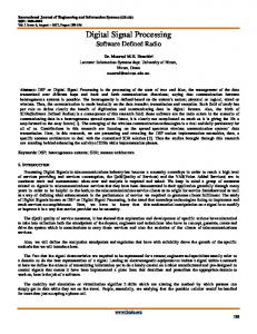
Research Article A SystemC-Based Design Methodology for Digital Signal Processing Systems ¨ Christian Haubelt, Joachim Falk, Joachim Keinert, Thomas Schlichter, Martin Streubuhr, Andreas Deyhle, ¨ Andreas Hadert, and Jurgen Teich Hardware-Software-Co-Design, Department of Copmuter Sciences, Friedrich-Alexander-University of Erlangen-Nuremberg, 91054 Erlangen, Germany Received 7 July 2006; Revised 14 December 2006; Accepted 10 January 2007 Recommended by Shuvra Bhattacharyya Digital signal processing algorithms are of big importance in many embedded systems. Due to complexity reasons and due to the restrictions imposed on the implementations, new design methodologies are needed. In this paper, we present a SystemC-based solution supporting automatic design space exploration, automatic performance evaluation, as well as automatic system generation for mixed hardware/software solutions mapped onto FPGA-based platforms. Our proposed hardware/software codesign approach is based on a SystemC-based library called SysteMoC that permits the expression of different models of computation well known in the domain of digital signal processing. It combines the advantages of executability and analyzability of many important models of computation that can be expressed in SysteMoC. We will use the example of an MPEG-4 decoder throughout this paper to introduce our novel methodology. Results from a five-dimensional design space exploration and from automatically mapping parts of the MPEG-4 decoder onto a Xilinx FPGA platform will demonstrate the effectiveness of our approach. Copyright © 2007 Christian Haubelt et al. This is an open access article distributed under the Creative Commons Attribution License, which permits unrestricted use, distribution, and reproduction in any medium, provided the original work is properly cited.

1.

INTRODUCTION

Digital signal processing algorithms, as for example real-time image enhancement, scene interpretation, or audio and video coding, have gained enormous popularity in embedded system design. They encompass a large variety of different algorithms, starting from simple linear filtering up to entropy encoding or scene interpretation based on neuronal networks. Their implementation, however, is very laborious and time consuming, because many different and often conflicting criteria must be met, as for example high throughput and low power consumption. Due to this rising complexity of these digital signal processing applications, there is demand for new design automation tools at a high level of abstraction. Many design methodologies are proposed in the literature for exploring the design space of implementations of digital signal processing algorithms (cf. [1, 2]), but none of them is able to fully automate the design process. In this paper, we will close this gap by proposing a novel approach based on SystemC [3–5], a C++ class library, and state-ofthe-art design methodologies. The proposed approach permits the design of digital signal processing applications with

minimal designer interaction. The major advantage with respect to existing approaches is the combination of executability of the specification, exploration of implementation alternatives, and the usability of formal analysis techniques for restricted models of computation. This is achieved through restricting SystemC such that we are able to automatically detect the underlying model of computation (MoC) [6]. Our design methodology comprises the automatic design space exploration using state-of-the-art multiobjective evolutionary algorithms, the performance evaluation by automatically generating efficient simulation models, and automatic platformbased system generation. The overall design flow as proposed in this paper is shown in Figure 1 and is currently implemented in the framework SystemCoDesigner. Starting with an executable specification written in SystemC, the designer can specify the target architecture template as well as the mapping constraints of the SystemC modules. In order to automate the design process, the SystemC application has to be written in a synthesizable subset of SystemC, called SysteMoC [7], and the target architecture template must be built from components supported by our component library. The components in the component

2

EURASIP Journal on Embedded Systems Architecture template

Mapping constraints

Sp

eci

Specifi

fie s es

Se

lec

ts

Application

Multiobjective optimization Communication library

Performance evaluation

Implementation

Component library Selec ts

System generation

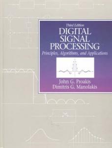
Figure 1: SystemCoDesigner design flow: for a given executable specification written in SystemC, the designer has to specify the architecture template as well as mapping constraints. The design space exploration is performed automatically using multiobjective evolutionary algorithms and is guided by an automatic simulation-based performance evaluation. Finally, any selected implementation can be automatically mapped efficiently onto an FPGA-based platform.

library are either written by hand using a hardware description language or can be taken from third party vendors. In this work, we will use IP cores especially provided by Xilinx. Furthermore, it is also possible to synthesize SysteMoC actors to RTL Verilog or VHDL using high-level synthesis tools as Mentor CatapultC [8] or Forte Cynthesizer [9]. However, there are limitations imposed on the actors given by these tools. As this is beyond the scope of this paper, we will omit discussing these issues here. With this specification, the SystemCoDesigner design process is automated as much as possible. Inside SystemCoDesigner, a multiobjective evolutionary optimization (MOEA) strategy is used in order to perform design space exploration. The exploration is guided by a simulation-based performance evaluation. Using SysteMoC as a specification language for the application, the generation of the simulation model inside the exploration can be automated. Then, the designer can carry out the decision making and select a design point for implementation. Finally, the platform-based implementation is generated automatically. The remainder of this paper is dedicated to the different issues arising during our proposed design flow. Section 3 discusses the input format based on SystemC called SysteMoC. SysteMoC is a library based on SystemC that allows to describe and simulate communicating actors. The particularity of this library for actor-based design is to separate actor functionality and communication behavior. In particular, the separation of actor firing rules and communication behavior

is achieved by an explicit finite state machine model associated with each actor. This finite state machine permits the identification of the underlying model of computation of the SystemC application and, hence, if possible, allows to analyze the specification with formal techniques for properties such as boundedness of memory, (periodic) schedulability, deadlocks, and so forth. Section 4 presents the model and the tasks performed during design space exploration. As the SysteMoC description only models the specified behavior of our system, we need additional information in order to perform system-level synthesis. Following the Y-chart approach [10, 11], a formal model of architecture (MoA) must be specified by the designer as well as mapping constraints for the actors in the SysteMoC description. With this formal model the systemlevel synthesis task is twofold: (1) determine the allocation of resources from the architecture template and (2) determine a binding of SystemC modules (actors) onto the allocated resources. During design space exploration, many implementations are constructed by the system-level exploration tool SystemCoDesigner. Each resulting implementation must be evaluated regarding different properties such as area, power consumption, performance, and so forth. Especially the performance evaluation, that is, latency and throughput, is critical in the context of digital signal processing applications. In our proposed methodology, we will use, beside others, a simulation-based approach. We will show how SysteMoC might help to automatically generate efficient simulation models during exploration. In Section 5 our approach to automatic platform-based system synthesis will be presented targeting in our examples a Xilinx Virtex-II Pro FPGA-based platform. The key idea is to generate a platform, perform software synthesis, and provide efficient communication channels for the implementation. The results obtained by the synthesis will be compared to the simulation models generated during a fivedimensional design space exploration in Section 6. We will use the example of an MPEG-4 decoder throughout this paper to present our methodology. 2.

RELATED WORK

In this section, we discuss some tools which are available for the design and synthesis of digital signal processing algorithms onto mixed and possibly multicore system-on-achip (SoC). Sesame (simulation of embedded system architectures for multilevel exploration) [12] is a tool for performance evaluation and exploration of heterogeneous architectures for the multimedia application domain. The applications are given by Kahn process networks modeled with a C++ class library. The architecture is modeled by architecture building blocks taken from a library. Using a SystemCbased simulator at transaction level, performance evaluation can be done for a given application. In order to cosimulate the application and the architecture, a trace-driven simulation approach technique is chosen. Sesame is developed in the context of the Artemis project (architectures and methods for embedded media systems) [13].

Christian Haubelt et al. The MILAN (model-based integrated simulation) framework is a design space exploration tool that works at different levels of abstraction [14]. Following the Y-chart approach [11], MILAN uses hierarchical dataflow graphs including function alternatives. The architecture template can be defined at different levels of detail. The hierarchical design space exploration starts at the system level and uses rough estimation and symbolic methods based on ordered binary decision diagrams to prune the search space. After reducing the search space, a more fine grained estimation is performed for the remaining designs, reducing the search space even more. At the end, at most ten designs are evaluated by cycleaccurate trace-driven simulation. MILAN needs user interaction to perform decision making during exploration. In [15], Kianzad and Bhattacharyya propose a framework called CHARMED (cosynthesis of hardware-software multimode embedded systems) for the automatic design space exploration for periodic multimode embedded systems. The input specification is given by several task graphs where each task graph is associated to one of M modes. Moreover, a period for each task graph is given. Associated with the vertices and edges in each task graph, there are attributes like memory requirement and worst case execution time. Two kinds of resources are distinguished, processing elements and communication resources. Kianzad and Bhattacharyya use an approach based on SPEA2 [16] with constraint dominance, a similar optimization strategy as implemented by our SystemCoDesigner. Balarin et al. [17] propose Metropolis, a design space exploration framework which integrates tools for simulation, verification, and synthesis. Metropolis is an infrastructure to help designers to cope with the difficulties in large system designs by allowing the modeling on different levels of detail and supporting refinement. The applications are modeled by a metamodel consisting of sequential processes communicating via the so-called media. A medium has variables and functions where the variables are only allowed to be changed by the functions. From the application model a sequence of event vectors is extracted representing a partial execution order. Nondeterminism is allowed in application modeling. The architecture again is modeled by the metamodel, where media are resources and processes representing services (a collection of functions). Deriving the sequence of event vectors results in a nondeterministic execution order of all functions. The mapping is performed by intersecting both event sequences. Scheduling decisions on shared resources are resolved by the so-called quantity managers which annotate the events. That way, quantity managers can also be used to associate other properties with events, like power consumption. In contrast to SystemCoDesigner, Metropolis is not concerned with automatic design space exploration. It supports refinement and abstraction, thus allowing top-down and bottom-up methodologies with a meet in the middle approach. As Metropolis is a framework based on a metamodel implementing the Y-chart approach, many system-level design methodologies, including SystemCoDesigner, may be represented in Metropolis.

3 Finally, some approaches exist to map digital signal processing algorithms automatically to an FPGA platform. Compaan/Laura [18] automatically converts a Matlab loop program into a KPN network. This process network can be transformed into a hardware/software system by instantiating IP cores and connecting them with FIFOs. Special software routines take care of the hardware/software communication. Whereas [18] uses a computer system together with a PCI FPGA board for implementation, [19] automates the generation of a SoC (system on chip). For this purpose, the user has to provide a platform specification enumerating the available microprocessors and communication infrastructure. Furthermore, a mapping has to be provided specifying which process of the KPN graph is executed on which processor unit. This information allows the ESPAM tool to assemble a complete system including different communication modules as buses and point-to-point communication. The Xilinx EDK tool is used for final bitstream generation. Whereas both Compaan/Laura/ESPAM and SystemCoDesigner want to simplify and accelerate the design of complex hardware/software systems, there are significant differences. First of all, Compaan/Laura/ESPAM uses Matlab loop programs as input specification, whereas SystemCoDesigner bases on SystemC allowing for both simulation and automatic hardware generation using behavioral compilers. Furthermore, our specification language SysteMoC is not restricted to KPN, but allows to represent different models of computation. ESPAM provides a flexible platform using generic communication modules like buses, cross-bars, point-to-point communication, and a generic communication controller. SystemCoDesigner currently restricts to extended FIFO communication allowing out-of-order reads and writes. Additionally our approach tightly includes automatic design space exploration, estimating the achievable system performance. Starting from an architecture template, a subset of resources is selected in order to obtain an efficient implementation. Such a design point can be automatically translated into a system on chip. Another very interesting approach based on UML is presented in [20]. It is called Koski and as SystemCoDesigner, it is dedicated to the automatic SoC design. Koski follows the Y-chart approach. The input specification is given as Kahn process networks modeled in UML. The Kahn processes are modeled using Statecharts. The target architecture consists of the application software, the platformdependent and platform-independent software, and synthesizable communication and processing resources. Moreover, special functions for application distribution are included, that is, interprocess communication for multiprocessor systems. During design space exploration, Koski uses simulation for performance evaluation. Also, Koski has many similarities with SystemCoDesigner, there are major differences. In comparison to SystemCoDesigner, Koski has the following advantages. It supports a network communication which is more platform-independent than the SystemCoDesigner approach. It is also somehow more flexible

4 by supporting a real-time operating System (RTOS) on the CPU. However, there are many advantages when using SystemCoDesigner. (1) SystemCoDesigner permits the specification directly in SystemC and automatically extracts the underlying model of computation. (2) The architecture specification in SystemCoDesigner is not limited to a shared communication medium, it also allows for optimized point-to-point communication. The main advantage of the SystemCoDesigner is its multiobjective design space exploration which allows for optimizing several objectives simultaneously. The Ptolemy II project [21] was started in 1996 by the University of California, Berkeley. Ptolemy II is a software infrastructure for modeling, analysis, and simulation of embedded systems. The focus of the project is on the integration of different models of computation by the so-called hierarchical heterogeneity. Currently, supported MoCs are continuous time, discrete event, synchronous dataflow, FSM, concurrent sequential processes, and process networks. By coupling different MoCs, the designer has the ability to model, analyze, or simulate heterogeneous systems. However, as different actors in Ptolemy II are written in JAVA, it is limited in its usability of the specification for generating efficient hardware/software implementations including hardware and communication synthesis for SoC platforms. Moreover, Ptolemy II does not support automatic design space exploration. The Signal Processing Worksystem (SPW) from Cadence Design Systems, Inc., is dedicated to the modeling and analysis of signal processing algorithms [22]. The underlying model is based on static and dynamic dataflow models. A hierarchical composition of the actors is supported. The actors themselves can be specified by several different models like SystemC, Matlab, C/C++, Verilog, VHDL, or the design library from SPW. The main focus of the design flow is on simulation and manual refinement. No explicit mapping between application and architecture is supported. CoCentric System Studio is based on languages like C/C++, SystemC, VHDL, Verilog, and so forth, [23]. It allows for algorithmic and architecture modeling. In System Studio, algorithms might be arbitrarily nested dataflow models and FSMs [24]. But in contrast to Ptolemy II, CoCentric allows hierarchical as well as parallel combinations, what reduces the analysis capability. Analysis is only supported for pure dataflow models (deadlock detection, consistency) and pure FSMs (causality). The architectural model is based on the transaction-level model of SystemC and permits the inclusion of other RTL models as well as algorithmic System Studio models and models from Matlab. No explicit mapping between application and architecture is given. The implementation style is determined by the actual encoding a designer chooses for a module. Beside the modeling and design space exploration aspects, there are several approaches to efficiently represent MoCs in SystemC. The facilities for implementing MoCs in SystemC have been extended by Herrera et al. [25] who have implemented a custom library of channel types like rendezvous on top of the SystemC discrete event simulation ker-

EURASIP Journal on Embedded Systems nel. But no constraints have imposed how these new channel types are used by an actor. Consequently, no information about the communication behavior of an actor can be automatically extracted from the executable specification. Implementing these channels on top of the SystemC discrete event simulation kernel curtails the performance of such an implementation. To overcome these drawbacks, Patel and Shukla [26–28] have extended SystemC itself with different simulation kernels for communicating sequential processes (CSP), continuous time (CT), dataflow process networks (PN) dynamic as well as static (SDF), and finite state machine (FSM) MoCs to improve the simulation efficiency of their approach. 3.

EXPRESSING DIFFERENT MoCs IN SYSTEMC

In this section, we will introduce our library-based approach to actor-based design called SysteMoC [7] which is used for modeling the behavior and as synthesizable subset of SystemC in our SystemCoDesigner design flow. Instead of a monolithic approach for representing an executable specification as done using many design languages, SysteMoC supports an actor-oriented design [29, 30] for many dataflow models of computation (MoCs). These models have been applied successfully in the design of digital signal processing algorithms. In this approach, we consider timing and functionality to be orthogonal. Therefore, our design must be modeled in an untimed dataflow MoC. The timing of the design is derived in the design space exploration phase from mapping of the actors to selected resources. Note that the timing given by that mapping in general affects the execution order of actors. In Section 4, we present a mechanism to evaluate the performance of our application with respect to a candidate architecture. On the other hand, industrial design flows often rely on executable specifications, which have been encoded in design languages which allow unstructured communication. In order to combine both approaches, we propose the SysteMoC library which permits writing an executable specification in SystemC while separating the actor functionality from the communication behavior. That way, we are able to identify different MoCs modeled in SysteMoC. This enables us to represent different algorithms ranging from simple static operations modeled by homogeneous synchronous dataflow (HSDF) [31] up to complex, data-dependent algorithms as run-length entropy encoding modeled as Kahn process networks (KPN) [32]. In this paper, an MPEG-4 decoder [33] will be used to explain our system design methodology which encompasses both algorithm types and can hence only be modeled by heterogeneous models of computation. 3.1.

Actor-oriented model of an MPEG-4 decoder

In actor-oriented design, actors are objects which execute concurrently and can only communicate with each other via channels instead of method calls as known in object-oriented design. Actor-oriented designs are often represented by bipartite graphs consisting of channels c ∈ C and actors a ∈ A, which are connected via point-to-point connections from an

Christian Haubelt et al.

5 Output port o1

a1 |FileSrc

o1 c i1 1

Channel a6 |FileSnk

i1

c8

o1

o1

a2 |Parser o2 c7 i3

c2

i1

a3 |Recon o2

c6 o2

a5 |MComp

i1

c5

o1

a|Scale fscale

o1 c4

c3 i2

Functionality a.F

i2

i1

Activation pattern

a4 |IDCT2D i1

Actor instance a5 of actor type “MComp”

i1 (1)&o1 (1) / fscale t1

Action o1

sstart

Input port i1 Input port a.I = {i1 }

Figure 2: The network graph of an MPEG-4 decoder. Actors are shown as boxes whereas channels are drawn as circles.

actor output port o to a channel and from a channel to an actor input port i. In the following, we call such representations network graphs. These network graphs can be extracted directly from the executable SysteMoC specification. Figure 2 shows the network graph of our MPEG-4 decoder. MPEG-4 [33] is a very complex object-oriented standard for compression of digital videos. It not only encompasses the encoding of the multimedia content, but also the transport over different networks including quality of service aspects as well as user interaction. For the sake of clarity, our decoder implementation restricts to the decompression of a basic video bit-stream which is already locally available. Hence, no transmission issues must be taken into account. Consequently, our bit-stream is read from a file by the FileSrc actor a1 , where a1 ∈ A identifies an actor from the set of all actors A. The Parser actor a2 analyzes the provided bit-stream and extracts the video data including motion compensation vectors and quantized zig-zag encoded image blocks. The latter ones are forwarded to the reconstruction actor a3 which establishes the original 8 × 8 blocks by performing an inverse zig-zag scanning and a dequantization operation. From these data blocks the two-dimensional inverse cosine transform actor a4 generates the motion-compensated difference blocks. They are processed by the motion compensation actor a5 in order to obtain the original image frame by taking into account the motion compensation vectors provided by the Parser actor. The resulting image is finally stored to an output file by the FileSnk actor a6 . In the following, we will formally present the SysteMoC modeling concepts in detail. 3.2. SysteMoC concepts The network graph is the usual representation of an actororiented design. It consists of actors and channels, as seen in Figure 2. More formally, we can derive the following definition. Definition 1 (network graph). A network graph is a directed bipartite graph gn = (A, C, P, E) containing a set of actors A, a set of channels C, a channel parameter function P : C → N∞ × V ∗ which associates with each channel c ∈ C its buffer size n ∈ N∞ = {1, 2, 3, . . . ,∞}, and also a possibly nonempty sequence v ∈ V ∗ of initial tokens, where

Output port a.O = {o1 }

Firing FSM a.R of actor instance a

Figure 3: Visual representation of the Scale actor as used in the IDCT2D network graph displayed in Figure 4. The Scale actor is composed of input ports and output ports, its functionality, and the firing FSM determining the communication behavior of the actor.

V ∗ denotes the set of all possible finite sequences of tokens v ∈ V [6]. Additionally, the network graph consists of directed edges e ∈ E ⊆ (C × A.I) ∪ (A.O × C) between actor output ports o ∈ A.O and channels as well as channels and actor input ports i ∈ A.I. These edges are further constraints such that each channel can only represent a point-to-point connection, that is, exactly one edge is connected to each actor port and the in-degree and out-degree of each channel in the graph are exactly one. Actors are used to model the functionality. An actor a is only permitted to communicate with other actors via its actor ports a.P .1 Other forms of interactor communication are forbidden. In this sense, a network graph is a specialization of the framework concept introduced in [29], which can express an arbitrary connection topology and a set of initial states. Therefore, the corresponding set of framework states Σ is given by the product set of all possible sequences of all channels of the network graph and the single initial state is derived from the channel parameter function P. Furthermore, due to the point-to-point constraint of a network graph, two framework actions λ1 , λ2 referenced in different framework actors are constrained to only modify parts of the framework state corresponding to different network graph channels. Our actors are composed from actions supplying the actor with its data transformation functionality and a firing FSM encoding, the communication behavior of the actor, as illustrated in Figure 3. Accordingly, the state of an actor is also divided into the functionality state only modified by the actions and the firing state only modified by the firing FSM. As actions do not depend on or modify the framework state 1

We use the “.”-operator, for example, a.P , for denoting member access, for example, P , of tuples whose members have been explicitly named in their definition, for example, a ∈ A from Definition 2. Moreover, this member access operator has a trivial pointwise extension to sets of tuples,  for example, A.P = a∈A a.P , which is also used throughout this paper.

6 their execution corresponds to a sequence of internal transitions as defined in [29]. Thus, we can define an actor as follows. Definition 2 (actor). An actor is a tuple a = (P , F , R) containing a set of actor ports P = I ∪ O partitioned into actor input ports I and actor output ports O, the actor functionality F and the firing finite state machine (FSM) R. The notion of the firing FSM is similar to the concepts introduced in FunState [34] where FSMs locally control the activation of transitions in a Petri Net. In SysteMoC, we have extended FunState by allowing guards to check for available space in output channels before a transition can be executed. The states of the firing FSM are called firing states, directed edges between these firing states are called firing transitions, or transitions for short. The transitions are guarded by activation patterns k = kin ∧ kout ∧ kfunc consisting of (i) predicates kin on the number of available tokens on the input ports called input patterns, for example, i(1) denotes a predicate that tests the availability of at least one token on the actor input port i, (ii) predicates kout on the number of free places on the output ports called output patterns, for example, o(1) checks if the number of free places of an output is at least one, and (iii) more general predicates kfunc called functionality conditions depending on the functionality state, defined below, or the token values on the input ports. Additionally, the transitions are annotated with actions defining the actor functionality which are executed when the transitions are taken. Therefore, a transition corresponds to a precise reaction as defined in [29], where an input/output pattern corresponds to an I/O transition in the framework model. And an activation pattern is always a responsible trigger, as actions correspond to a sequence of internal transitions, which are independent from the framework state. More formally, we derive the following two definitions. Definition 3 (firing FSM). The firing FSM of an actor a ∈ A is a tuple a.R = (T, Qfiring , q0 firing ) containing a finite set of firing transitions T, a finite set of firing states Qfiring , and an initial firing state q0 firing ∈ Qfiring . Definition 4 (transition). A firing transition is a tuple t = (qfiring , k, faction , qfiring ) ∈ T containing the current firing state qfiring ∈ Qfiring , an activation pattern k = kin ∧ kout ∧ kfunc , the associated action faction ∈ a.F , and the next firing state ∈ Qfiring . The activation pattern k is a Boolean funcqfiring tion which determines if transition t can be taken (true) or not (false). The actor functionality F is a set of methods of an actor partitioned into actions used for data transformation and guards used in functionality conditions of the activation pattern, as well as the internal variables of the actor, and their initial values. The values of the internal variables of an actor are called its functionality state qfunc ∈ Qfunc and their initial values are called the initial functionality state q0 func . Actions and guards are partitioned according to two fundamental

EURASIP Journal on Embedded Systems differences between them: (i) a guard just returns a Boolean value instead of computing values of tokens for output ports, and (ii) a guard must be side-effect free in the sense that it must not be able to change the functionality state. These concepts can be represented more formally by the following definition. Definition 5 (functionality). The actor functionality of an actor a ∈ A is a tuple a.F = (F, Qfunc , q0 func ) containing a set of functions F = Faction ∪ Fguard partitioned into actions and guards, a set of functionality states Qfunc (possibly infinite), and an initial functionality state q0 func ∈ Qfunc . Example 1. To illustrate these definitions, we give the formal representation of the actor a shown in Figure 3. As can be seen the actor has two ports, P = {i1 , o1 }, which are partitioned into its set of input ports, I = {i1 }, and its set of output ports, O = {o1 }. Furthermore, the actor contains exactly one method F .Faction = { fscale }, which is the action fscale : V × Qfunc → V × Qfunc for generating token v ∈ V containing scaled IDCT values for the output port o1 from values received on the input port i1 . Due to the lack of any internal variables, as seen in Example 2, the set of functionality states Qfunc = {q0 func } contains only the initial functionality state q0 func encoding the scale factor of the actor. The execution of SysteMoC actors can be divided into three phases. (i) Checking for enabled transitions t ∈ T in the firing FSM R. (ii) Selecting and executing one enabled transition t ∈ T which executes the associated actor functionality. (iii) Consuming tokens on the input ports a.I and producing tokens on the output ports a.O as indicated by the associated input and output patterns t.kin and t.kout . 3.3.

Writing actors in SysteMoC

In the following, we describe the SystemC representation of actors as defined previously. SysteMoC is a C++ class library based on SystemC which provides base classes for actors and network graphs as well as operators for declaring firing FSMs for these actors. In SysteMoC, each actor is represented as an instance of an actor class, which is derived from the C++ base class smoc actor, for example, as seen in Example 2, which describes the SysteMoC implementation of the Scale actor already shown in Figure 3. An actor can be subdivided into three parts: (i) actor input ports and output ports, (ii) actor functionality, and (iii) actor communication behavior encoded explicitly by the firing FSM. Example 2. SysteMoC code for the Scale actor being part of the MPEG-4 decoder specification. 00 class Scale: public smoc_actor { 01 public: 02 // Input port declaration 03 smoc_port_in i1; 04 // Output port declaration 05 smoc_port_out o1; 06 private:

Christian Haubelt et al. 07 // Actor parameters 08 const int G, OS; 09 10 // functionality 11 void scale() { o1[0] = OS 12 + (G * i1[0]); } 13 14 // Declaration of firing FSM states 15 smoc_firing_state start; 16 public: 17 // The actor constructor is responsible 18 // for declaring the firing FSM and 19 // initializing the actor 20 Scale(sc_module_name name, int G, int OS) 21 : smoc_actor(name, start), 22 G(G), OS(OS) { 23 // start state consists of 24 // a single self loop 25 start = 26 // input pattern requires at least 27 // one token in the FIFO connected 28 // to input port i1 29 (i1.getAvailableTokens() >= 1) >> 30 // output pattern requires at least 31 // space for one token in the FIFO 32 // connected to output port o1 33 (o1.getAvailableSpace() >= 1) >> 34 // has action Scale::scale and 35 // next state start 36 CALL(Scale::scale) >> 37 start; 38 } 39 }; As known from SystemC, we use port declarations as shown in lines 2-5 to declare the input and output ports a.P for the actor to communicate with its environment. Note that the usage of sc fifo in and sc fifo out ports as provided by the SystemC library would not allow the separation of actor functionality and communication behavior as these ports allow the actor functionality to consume tokens or produce tokens, for example, by calling read or write methods on these ports, respectively. For this reason, the SysteMoC library provides its own input and output port declarations smoc port in and smoc port out. These ports can only be used by the actor functionality to peek token values already available or to produce tokens for the actual communication step. The token production and consumption is thus exclusively controlled by the local firing FSM a.R of the actor. The functions f ∈ F of the actor functionality a.F and its functionality state qfunc ∈ Qfunc are represented by the class methods as shown in line 11 and by class member variables (line 8), respectively. The firing FSM is constructed in the constructor of the actor class, as seen exemplarily for a single transition in lines 25–37. For each transition t ∈ R.T, the number of required input tokens, the quantity of produced output tokens, and the called function of the actor functionality are indicated by the help of the methods

7 getAvailableTokens(), getAvailableSpace(), and CALL(), respectively. Moreover, the source and sink state of the firing FSM are defined by the C++-operators = and >>. For a more detailed description of the firing FSM syntax, see [7]. 3.4.

Application modeling using SysteMoC

In the following, we will give an introduction to different MoCs well known in the domain of digital signal processing and their representation in SysteMoC by presenting the MPEG-4 application in more detail. As explained earlier in this section, MPEG-4 is a good example of today’s complex signal processing applications. They can no longer be modeled at a granularity level sufficiently detailed for design space exploration by restrictive MoCs like synchronous dataflow (SDF) [35]. However, as restrictive MoCs offer better analysis opportunities they should not be discarded for subsystems which do not need more expressiveness. In our SysteMoC approach, all actors are described by a uniform modeling language in such a way that for a considered group of actors it can be checked whether they fit into a given restricted MoC. In the following, these principles are shown exemplarily for (i) synchronous dataflow (SDF), (ii) cyclostatic dataflow (CSDF) [36], and (iii) Kahn process networks (KPN) [32]. Synchronous dataflow (SDF) actors produce and consume upon each invocation a static and constant amount of tokens. Hence, their external behavior can be determined statically at compile time. In other words, for a group of SDF actors, it is possible to generate a static schedule at compile time, avoiding the overhead of dynamic scheduling [31, 37, 38]. For homogeneous synchronous dataflow, an even more restricted MoC where each actor consumes and produces exactly one token per invocation and input (output), it is even possible to efficiently compute a rate-optimal buffer allocation [39]. The classification of SysteMoC actors is performed by comparing the firing FSM of an actor with different FSM templates, for example, single state with self loop corresponding to the SDF domain or circular connected states corresponding to the CSDF domain. Due to the SysteMoC syntax discussed above, this information can be automatically derived from the C++ actor specification by simply extracting the firing FSM specified in the actor. More formally, we can derive the following condition: given an actor a = (P , F , R), the actor can be classified as belonging to the SDF domain if each transition has the same input pattern and output pattern, that is, for all t1 , t2 ∈ R.T : t1 .kin ≡ t2 .kin ∧ t1 .kout ≡ t2 .kout . Our MPEG-4 decoder implementation contains various such actors. Figure 3 represents the firing FSM of a scaler actor which is a simple SDF actor. For each invocation, it reads a frequency coefficient and multiplies it with a constant gain factor in order to adapt its range. Cyclo-static dataflow (CSDF) actors are an extension of SDF actors because their token consumption and production do not need to be constant but can vary cyclically. For this purpose, their execution is divided into a fixed number

EURASIP Journal on Embedded Systems

Scale1

AddSub6

Fly1

AddSub3

AddSub7

Fly2

AddSub4

AddSub8

Fly3

AddSub5

o1

i1

Sink 8 × 8

ToBlock

i1–8

o1–8

Clip

i1–8

i1–8

IDCT-1D2 o1–8

o1–8

i9

AddSub2

Scale2

AddSub1

i1–8

IDCT-1D1 o1–8

i1–8

o1–8

i1

o1

Transpose

IDCT2D for 8 × 8 blocks

o2 ToRows

Src 8 × 8 + max value

8

AddSub9

AddSub10

Figure 4: The displayed network graph is the hierarchical refinement of the IDCT2D actor a4 from Figure 2. It implements a two-dimensional inverse cosine transformation (IDCT) on 8 × 8 blocks of pixels. As can be seen in the figure, the two-dimensional inverse cosine transformation is composed of two one-dimensional inverse cosine transformations IDCT-1D1 and IDCT-1D2 .

of phases which are repeated periodically. In each phase, a constant number of tokens is written to or read from each actor port. Similar to SDF graphs, a static schedule can be generated at compile time [40]. Although many CSDF graphs can be translated to SDF graphs by accumulating the token consumption and production rates for each actor over all phases, their direct implementation leads mostly to less memory consumption [40]. In our MPEG-4 decoder, the inverse discrete cosine transformation (IDCT), as shown in Figure 4, is a candidate for static scheduling. However, due to the CSDF actor Transpose it cannot be classified as an SDF subsystem. But the contained one-dimensional IDCT is an example of an SDF subsystem, only consisting of actors which satisfy the previously given constraints. An example of such an actor is shown in Figure 3. An example of a CSDF actor in our MPEG-4 application is the Transpose actor shown in Figure 4 which swaps rows and columns of the 8 × 8 block of pixels. To expose more parallelism, this actor operates on rows of 8 pixels received in parallel on its 8 input ports i1–8 , instead of whole 8 × 8 blocks, forcing the actor to be a CSDF actor with 8 phases for each of the 8 rows of a 8 × 8 block. Note that the CSDF actor Transpose is represented in SysteMoC by a firing FSM which contains exactly as many circularly connected firing states as the CSDF actor has execution phases. However, more complex firing FSMs can also exhibit CSDF semantic, for example, due to redundant states in the firing FSM or transitions with the same input and output patterns, the same source and destination firing state but different functionality conditions and actions. Therefore, CSDF actor classification should be performed on a transformed

firing FSM, derived by discarding the action and functionality conditions from the transitions and performing FSM minimization. More formally, we can derive the following condition: given an actor a = (P , F , R), the actor can be classified as belonging to the CSDF domain if exactly one transition is leaving and entering each firing state, that is, for all q ∈ R.Qfiring : |{t ∈ R.T | t.qfiring = q}| = 1 ∧ |{t ∈ R.T | t.qfiring = q}| = 1, and each state of the firing FSM is reachable from the initial state. Kahn process networks (KPN) can also be modeled in SysteMoC by the use of more general functionality conditions in the activation patterns of the transitions. This allows to represent data-dependent operations, for example, as needed by the bit-stream parsing as well as the decoding of the variable length codes in the Parser actor. This is exemplarily shown for some transitions of the firing FSM in the Parser actor of the MPEG-4 decoder in order to demonstrate the syntax for using guards in the firing FSM of an actor. The actions cannot determine presence or absence of tokens, or consume or produce tokens on input or output channels. Therefore, the blocking reads of the KPN networks are represented by the blocking behavior of the firing FSM until at least one transition leaving the current firing state is enabled. The behavior of Kahn process networks must be independent from the scheduling strategy. But the scheduling strategy can only influence the behavior of an actor if there is a choice to execute one of the enabled transitions leaving the current state. Therefore, it is possible to determine if an actor a satisfies the KPN requirement by checking for the sufficient condition that all functionality conditions on all transitions leaving a firing state are mutually

Christian Haubelt et al. exclusive, that is, for all t1 , t2 ∈ a.R.T, t1 .qfiring = t2 .qfiring : for all qfunc ∈ a.F .Qfunc : t1 .kfunc (qfunc ) ⇒ ¬t2 .kfunc (qfunc ) ∧ t2 .kfunc (qfunc ) ⇒ ¬t1 .kfunc (qfunc ). This guarantees a deterministic behavior of the Kahn process network provided that all actions are also deterministic. Example 3. Simplified SysteMoC code of the firing FSM analyzing the header of an individual video frame in the MPEG4 bit-stream. 00 01 02 03 04 05 06 07 08 09 10 11 12 13 14 15 16 17 18 19 20 21 22 23 24 25 26 27 28 29 30 31 32 33 34 35 36 37 38

class Parser: public smoc actor { public: // Input port receiving MPEG-4 bit-stream smoc port in bits; ... private: // functionality ... // Declaration of guards bool guard vop start() const /∗ code here ∗/ bool guard vop done () const /∗ code here ∗/ ... // Declaration of firing FSM states smoc firing state vol, ..., vop2, vop3, ..., stuck; public: Parser(sc module name name) : smoc actor(name, vol) { ... vop2 = ((bits.getAvailableTokens() >= VOP START CODE LENGTH) && GUARD(&Parser::guard vop done)) >> CALL(Parser::action vop done) >> vol | ((bits.getAvailableTokens() >= VOP START CODE LENGTH) && GUARD(&Parser::guard vop start)) >> CALL(Parser::action vop start) >> vop3 | ((bits.getAvailableTokens() >= VOP START CODE LENGTH) && !GUARD(&Parser::guard vop done) && !GUARD(&Parser::guard vop start)) >> CALL(Parser::action vop other) >> stuck; ... // More state declarations } };

The data-dependent behavior of the firing FSM is implemented by the guards declared in lines 8-11. These functions can access the values of the input ports without consuming them or performing any other modifications of the functionality state. The GUARD()-method evaluates these guards during determination whether the transition is enabled or not.

9 4.

AUTOMATIC DESIGN SPACE EXPLORATION FOR DIGITAL SIGNAL PROCESSING SYSTEMS

Given an executable signal processing network specification written in SysteMoC, we can perform an automatic design space exploration (DSE). For this purpose, we need additional information, that is, a formal model for the architecture template as well as mapping constraints for the actors of the SysteMoC application. All these information are captured in a formal model to allow automatic DSE. The task of DSE is to find the best implementations fulfilling the requirements demanded by the formal model. As DSE is often confronted with the simultaneous optimization of many conflicting objectives, there is in general more than a single optimal solution. In fact, the result of the DSE is the so-called Pareto-optimal set of solutions [41], or at least an approximation of this set. Beside the task of covering the search space in order to guarantee good solutions, we have to consider the task of evaluating a single design point. In the design of FPGA implementations, the different objectives to minimize are, namely, the number of required look-up tables (LUTs), block RAMs (BRAMs), and flip-flops (FFs). These can be evaluated by analytic methods. However, in order to obtain good performance numbers for other especially important objectives such as latency and throughput, we will propose a simulation-based approach. In the following, we will present the formal model for the exploration, the automatic DSE using multiobjective evolutionary algorithms (MOEAs), as well as the concepts of our simulation-based performance evaluation. 4.1.

Design space exploration using MOEAs

For the automatic design space exploration, we provide a formal underpinning. In the following, we will introduce the so-called specification graph [42]. This model strictly separates behavior and system structure: the problem graph models the behavior of the digital signal processing algorithm. This graph is derived from the network graph, as defined in Section 3, by discarding all information inside the actors as described later on. The architecture template is modeled by the so-called architecture graph. Finally, the mapping edges associate actors of the problem graph with resources in the architecture graph by a “can be implemented by” relation. In the following, we will formalize this model by using the definitions given in [42] in order to define the task of design space exploration formally. The application is modeled by the so-called problem graph gp = (Vp , Ep ). Vertices v ∈ Vp model actors whereas edges e ∈ Ep ⊆ Vp × Vp represent data dependencies between actors. Figure 5 shows a part of the problem graph corresponding to the hierarchical refinement of the IDCT2D actor a4 from Figure 2. This problem graph is derived from the network graph by a oneto-one correspondence between network graph actors and channels to problem graph vertices while abstracting from

10

EURASIP Journal on Embedded Systems Problem graph Fly1

AddSub3

AddSub7

Fly2

AddSub4

AddSub8

F2

AS4

AS8

F1

AS3

AS7

OPB mB1 Architecture graph

Figure 5: Partial specification graph for the IDCT-1D actor as shown in Figure 4. The upper part is a part of the problem graph of the IDCT-1D. The lower part shows the architecture graph consisting of several dedicated resources {F1 , F2 , AS3 , AS4 , AS7 , AS8 } as well as a MicroBlaze CPU-core {mB1 } and an OPB (open peripheral bus [43]). The dashed lines denote the mapping edges.

actor ports, but keeping the connection topology, that is, ∃ f :gp .Vp → gn .A ∪ gn .C, f is a bijection : for all v1 , v2 ∈ gp .Vp : (v1 , v2 ) ∈ gp .Ep ⇔ ( f (v1 ) ∈ gn .C ⇒ ∃ p ∈ f (v2 ).I : ( f (v1 ), p) ∈ gn .E)∨( f (v2 ) ∈ gn .C ⇒ ∃ p ∈ f (v1 ).O :(p, f (v2 )) ∈ gn .E). The architecture template including functional resources, buses, and memories is also modeled by a directed graph termed architecture graph ga = (Va , Ea ). Vertices v ∈ Va model functional resources (RISC processor, coprocessors, or ASIC) and communication resources (shared buses or point-to-point connections). Note that in our approach, we assume that the resources are selected from our component library as shown in Figure 1. These components can be either written by hand in a hardware description language or can be synthesized with the help of high-level synthesis tools such as Mentor CatapultC [8] or Forte Cynthesizer [9]. This is a prerequisite for the later automatic system generation as discussed in Section 5. An edge e ∈ Ea in the architecture graph ga models a directed link between two resources. All the resources are viewed as potentially allocatable components. In order to perform an automatic DSE, we need information about the hardware resources that might by allocated. Hence, we annotate these properties to the vertices in the architecture graph ga . Typical properties are the occupied area by a hardware module or the static power dissipation of a hardware module. Example 4. For FPGA-based platforms, such as built on Xilinx FPGAs, typical resources are MicroBlaze CPU, open peripheral buses (OPB), fast simplex links (FSLs), or user specified modules representing implementations of actors in the problem graph. In the context of platform-based FPGA

designs, we will consider the number of resources a hardware module is assigned to, that is, for instance, the number of required look-up tables (LUTs), the number of required block RAMs (BRAMs), and the number of required flip-flops (FFs). Next, it is shown how user-defined mapping constraints representing possible bindings of actors onto resources can be specified in a graph-based model. Definition 6 (specification graph [42]). A specification graph gs (Vs , Es ) consists of a problem graph gp (Vp , Ep ), an architecture graph ga (Va , Ea ), and a set of mapping edges Em . In particular, Vs = Vp ∪ Va , Es = Ep ∪ Ea ∪ Em , where Em ⊆ Vp × Va . Mapping edges relate the vertices of the problem graph to vertices of the architecture graph. The edges represent userdefined mapping constraints in the form of the relation “can be implemented by.” Again, we annotate the properties of a particular mapping to an associated mapping edge. Properties of interest are dynamic power dissipation when executing an actor on the associated resource or the worst case execution time (WCET) of the actor when implemented on a CPU-core. In order to be more precise in the evaluation, we will consider the properties associated with the actions of an actor, that is, we annotate for each action the WCET to each mapping edge. Hence, our approach will perform an actoraccurate binding using an action-accurate performance evaluation, as discussed next. Example 5. Figure 5 shows an example of a specification graph. The problem graph shown in the upper part is a subgraph of the IDCT-1D problem graph from Figure 4. The architecture graph consists of several dedicated resources connected by FIFO channels as well as a MicroBlaze CPU-core and an on-chip bus called OPB (open peripheral bus [43]). The channels between the MicroBlaze and the dedicated resources are FSLs. The dashed edges between the two graphs are the additional mapping edges Em that describe the possible mappings. For example, all actors can be executed on the MicroBlaze CPU-core. For the sake of clarity, we omitted the mapping edges for the channels in this example. Moreover, we do not show the costs associated with the vertices in ga and the mapping edges to maintain clarity of the figure. In the above way, the model of a specification graph allows a flexible expression of the expert knowledge about useful architectures and mappings. The goal of design space exploration is to find optimal solutions which satisfy the specification given by the specification graph. Such a solution is called a feasible implementation of the specified system. Due to the multiobjective nature of this optimization problem, there is in general more than a single optimal solution. System synthesis Before discussing automatic design space exploration in detail, we briefly discuss the notion of a feasible implementation (cf. [42]). An implementation ψ = (α, β), being the result of

Christian Haubelt et al.

11

a system synthesis, consists of two parts: (1) the allocation α that indicates which elements of the architecture graph are used in the implementation and (2) the binding β, that is, the set of mapping edges which define the binding of vertices in the problem graph to resources of the architecture graph. The task of system synthesis is to determine optimal implementations. To identify the feasible region of the design space, it is necessary to determine the set of feasible allocations and feasible bindings. A feasible binding guarantees that communications demanded by the actors in the problem graph can be established in the allocated architecture. This property makes the resulting optimization problem hard to be solved. A feasible allocation is an allocation α that allows at least one feasible binding β. Example 6. Consider the case that the allocation of vertices in Figure 5 is given as α = {mB1 , OPB, AS3 , AS4 }. A feasible binding can be given by β = {(Fly1 , mB1 ), (Fly2 , mB1 ), (AddSub3 ,AS3 ), (AddSub4 ,AS4 ), (AddSub7 , mB1 ), (AddSub8 , mB1 )}. All channels in the problem graph are mapped onto the OPB. Given the implementation ψ, some properties of ψ can be calculated. This can be done analytically or simulationbased. The optimization problem Beside the problem of determining a single feasible solution, it is also important to identify the set of optimal solutions. This is done during automatic design space exploration (DSE). The task of automatic DSE can be formulated as a multiobjective combinatorial optimization problem. Definition 7 (automatic design space exploration). The task of automatic design space exploration is the following multiobjective optimization problem (see, e.g., [44]) where without loss of generality, only minimization problems are assumed here: minimize f (x), subject to : x represents a feasible implementation ψ, ci (x) ≤ 0, ∀i ∈ {1, . . . , q},

(1)

where x = (x1 , x2 , . . . , xm ) ∈ X is the decision vector, X is the decision space, f (x) = ( f1 (x), f2 (x), . . . , fn (x)) ∈ Y is the objective function, and Y is the objective space. Here, x is an encoding called decision vector representing an implementation ψ. Moreover, there are q constraints ci (x), i = 1, . . . , q, imposed on x defining the set of feasible implementations. The objective function f is n-dimensional, that is, n objectives are optimized simultaneously. For example, in embedded system design it is required that the monetary cost and the power dissipation of an implementation are minimized simultaneously. Often, objectives in embedded system design are conflicting [45].

Only those design points x ∈ X that represent a feasible implementation ψ and that satisfy all constraints ci are in the set of feasible solutions, or for short in the feasible set called Xf = {x | ψ(x) being feasible ∧ c(x) ≤ 0} ⊆ X. A decision vector x ∈ Xf is said to be nondominated regarding a set A ⊆ Xf if and only if a ∈ A : a  x with a  x if and only if for all i : fi (a) ≤ fi (x).2 A decision vector x is said to be Pareto optimal if and only if x is nondominated regarding Xf . The set of all Pareto-optimal solutions is called the Pareto-optimal set, or the Pareto set for short. We solve this challenging multiobjective combinatorial optimization problem by using the state-of-the-art MOEAs [46]. For this purpose, we use sophisticated decoding of the individuals as well as integrated symbolic techniques to improve the search speed [2, 42, 47–49]. Beside the task of covering the design space using MOEAs, it is important to evaluate each design point. As many of the considered objectives can be calculated analytically (e.g., FPGA-specific objectives such as total number of LUTs, FFs, BRAMs), we need in general more time-consuming methods to evaluate other objectives. In the following, we will introduce our approach to a simulation-based performance evaluation in order to assess an implementation by means of latency and throughput. 4.2.

Simulation-based performance evaluation

Many system-level design approaches rely on application modeling using static dataflow models of computation for signal processing systems. Popular dataflow models are SDF and CSDF or HSDF. Those models of computation allow for static scheduling [31] in order to assess the latency and throughput of a digital signal processing system. On the other hand, the modeling restrictions often prohibit the representation of complex real-world applications, especially if data-dependent control flow or data-dependent actor activation is required. As our approach is not limited to static dataflow models, we are able to model more flexible and complex systems. However, this implies that the performance evaluation in general is not any longer possible through static scheduling approaches. As synthesizing a hardware prototype for each design point is also too expensive and too time-consuming, a methodology for analyzing the system performance is needed. Generally, there exist two options to assess the performance of a design point: (1) by simulation and (2) by analytical methods. Simulation-based approaches permit a more detailed performance evaluation than formal analyses as the behavior and the timing can interfere as is the case when using nondeterministic merge actors. However, simulationbased approaches reveal only the performance for certain stimuli. In this paper, we focus on a simulation-based performance evaluation and we will show how to generate efficient SystemC simulation models for each design point during DSE automatically. Our performance evaluation concept is as follows: during design space exploration, we assess the performance of each 2

Without loss of generality, only minimization problems are considered.

12 feasible implementation with respect to a given set of stimuli. For this purpose, we also model the architecture in SystemC by means of the so-called virtual processing components [50]: for each activated vertex in the architecture graph, we create such a virtual processing component. These components are called virtual as they are not able to perform any computation but are only used to simulate the delays of actions from actors mapped onto these components. Thus, our simulation approach is called virtual processing components. In order to simulate the timing of the given SysteMoC application, the actors are mapped onto the virtual processing components according to the binding β. This is established by augmenting the end of all actions f ∈ a.F .Faction of each actor a ∈ gn .A with the so-called compute function calls. In the simulation, these function calls will block an actor until the corresponding virtual processing components signal the end of the computation. Note that this end time generally depends on (i) the WCET of an action, (ii) other actors bound onto the same virtual processing component, as well as (iii) the stimuli used for simulation. In order to simulate effects of resource contention and resolve resource conflicts, a scheduling strategy is associated with each virtual processing component. The scheduling strategy might be either preemptive or nonpreemptive, like first come first served, round robin, priority based [51]. Beside modeling WCETs of each action, we are able to model functional pipelining in our simulation approach. This is established by distinction of WCET and the so-called data introduction interval (DII). In this case, resource contention is only considered during the DII. The difference between WCET and DII is an additional delay for the production of output tokens of a computation and does not occupy any resources. Example 7. Figure 6 shows an example for modeling preemptive scheduling. Two actors, AddSub7 and AddSub8 , perform compute function calls on the instantiated MicroBlaze processor mB1 . We assume in this example that the MicroBlaze applied a priority-based scheduling strategy for scheduling all actor action execution requests that are bound to the MicroBlaze processor. We also assume that the actor AddSub7 has a higher priority than the actor AddSub8 . Thus, the execution of the action faddsub of the AddSub7 actor pre empts the execution of the action faddsub of the AddSub8 actor. Our VPC framework provides the necessary interface between virtual processing components and schedulers: the virtual processing component notifies the scheduler about each compute function call while the scheduler replies with its scheduling decision. The performance evaluation is performed by a combined simulation, that is, we simulate the functionality and the timing in one single simulation model. As a result of the SystemC-based simulation, we get traces logged during the simulation, showing the activation of actions, the start times, as well as the end times. These traces are used to assess the performance of an implementation by means of average latency and average throughput. In general, this approach leads

EURASIP Journal on Embedded Systems Functional model AddSub7

Architecture mapping

AddSub8

MicroBlaze mB1

compute ( faddsub )

ready

compute ( faddsub )

ready

return

block

return SysteMoC

Priority scheduler

block

SystemC/XML

Figure 6: Example of modeling preemptive scheduling within the concept of virtual processing components [50]: two actor actions compete for the same virtual processing component by compute function calls. An associated scheduler resolves the conflict by selecting the action to be executed.

to very precise simulation results according to the level of abstraction, that is, action accuracy. Compared to other approaches, we support a detailed performance evaluation of heterogeneous multiprocessor architectures supporting arbitrary preemptive and nonpreemptive scheduling strategies, while needing almost no source code modifications. The approach given in [52, 53] allows for modeling of real-time scheduling strategies by introducing a real-time operating system (RTOS) module based on SystemC. Therefore, each atomic operation, for example, any code line, is augmented by an await() function call within all software tasks. Each of those function calls enforces a scheduling decision, also known as cooperative scheduling. On top of those predetermined breaking points, the RTOS module emulates a preemptive scheduling policy for software tasks running on the same RTOS module. Another approach found in [54] motivates the socalled virtual processing units (VPU) for representing processors. Each VPU supports only a priority-based scheduling strategy. Software processes are modeled as timed communication extended finite state machines (tCEFSM). Each state transition of a tCEFSM represents an atomic operation and consumes a fixed amount of processor cycles. The modeling of time is the main limitation of this approach, because each transition of a tCEFSM requires the same number of processor cycles. Our VPC framework overcomes those limitations by combining (i) action-accurate, (ii) resourceaccurate, and (iii) contention- and scheduling-accurate timing simulation. In the Sesame framework [12] a virtual processor is used to map an event trace to a SystemC-based transaction level architecture simulation. For this purpose, the application

Christian Haubelt et al. code given as a Kahn process network is annotated with read, write, and execute statements. While executing the Kahn application, traces of application events are generated and passed to the virtual processor. Computational events (execute) are dispatched directly by the virtual processor which simulates the timing and communication events (read, write) are passed to a transaction level SystemC-based architecture simulator. As the scheduling of an event trace in a virtual processor does not affect the application, the Sesame framework does not support modeling of time-dependent application behavior. In our VPC framework, application and architecture are simulated in the same simulation-time domain and thus the blocking of a compute function call allows for simulation of time-dependent behavior. Further on, we do not explicitly distinguish between communication and computational execution, instead both types of execution use the compute function call for timing simulation. This abstract modeling of computation and communication delays results in a fast performance evaluation, but does not reveal the details of a transaction level simulation. One important aspect of our design flow is that we can generate these efficient simulation models automatically. This is due to our SysteMoC library.3 As we have to control the three phases in the simulation as discussed in Section 3.2, we can introduce the compute function calls directly at the end of phase (ii), that is, no additional modifications of the source code are necessary when using SysteMoC. In summary, the advantages of virtual processing components are (i) a clear separation between model of computation and model of architecture, (ii) a flexible mapping of the application to the architecture, (iii) a high level of abstraction, and (iv) the combination of functional simulation together with performance simulation. While performing design space exploration, there is a need for a rapid performance evaluation of different allocations α and bindings β. Thus, the VPC framework was designed for a fast simulation model generation. Figure 7 gives an overview of the implemented concepts. Figure 7(a) shows the implementation ψ = (α, β) as a result of the automatic design space exploration. In Figure 7(b), the automatically generated VPC simulation model is shown. The so-called Director is responsible for instantiating the virtual processing components according to a given allocation α. Moreover, the binding β is performed by the Director, in mapping each SysteMoC actor compute function call to the bound virtual processing components. Before running the simulation, the Director is configured with the necessary information, that is, implementation which should be evaluated. Finally, the Director manages the mapping parameters, that is, WCETs and DII of the actions in order to control the simulation times. The configuration is performed through an .xml-file omitting unnecessary recompilations of the simulation model for each design point and, thus, allowing for a fast performance evaluation of large populations of implementations. 3

VPC can also be used together with plain SystemC modules.

13 Problem graph Fly1

AddSub3

AddSub7

Fly2

AddSub4

AddSub8

F2 AS3

F1

mB1 Architecture graph (a) SysteMoC network graph Fly1

AddSub3

AddSub7

Fly2

AddSub4

AddSub8

Director

F2

mB1

C1

F2 Virtual processing components

Actor

compute

Component (b)

Figure 7: Approach to (i) action-accurate, (ii) resource-accurate, and (iii) contention- and scheduling-accurate simulation-based performance evaluation. (a) An example of one implementation as result of the automatic DSE, and (b) the corresponding VPC simulation model. The Director constructs the virtual processing components according to the allocation α. Additionally, the Director implements the binding of SysteMoC actors onto the virtual processing components according to a specific binding β.

5.

AUTOMATIC SYSTEM GENERATION

The result of the automatic design space exploration is a set of nondominated solutions. From these solutions, the designer can select one implementation according to additional requirements or preferences. This process is known as decision making in multiobjective optimization.

14 In this section, we show how to automatically generate a hardware/software implementation for FPGA-based SoC platforms according to the selected allocation and binding. For this purpose, three tasks must be performed: (1) generate the allocated hardware modules, (2) generate the necessary software for each allocated processor core including action code, communication code, and finally scheduling code, and (3) insert the communication resources establishing software/software, hardware/hardware, as well as hardware/software communication. In the following, we will introduce our solution to these three tasks. Moreover, the efficiency of our provided communication resources will be discussed in this section. 5.1. Generating the architecture Each implementation ψ = (α, β) produced by the automatic DSE and selected by the designer is used as input to our automatic system generator for FPGA-based SoC platforms. In our following case study, we specify the system generation flow for Xilinx FPGA platforms only. Figure 8 shows the general flow for Xilinx platforms. The architecture generation is threefold: first, the system generator automatically generates the MicroBlaze subsystems, that is, for each allocated CPU resource, a MicroBlaze subsystem is instantiated. Second, the system generator automatically inserts the allocated IP cores. Finally, the system generator automatically inserts the communication resources. The result of this architecture generation is a hardware description file (.mhs-file) in case of the Xilinx EDK (embedded development Kit [55]) toolchain. In the following, we discuss some details of the architecture generation process. According to these three above-mentioned steps, the resources in the architecture graph can be classified to be of type MicroBlaze, IP core, or Channel. In order to allow a hardware synthesis of this architecture, the vertices in the architecture graph contain additional information, as, for example, the memory sizes of the MicroBlazes or the names and versions of VHDL descriptions representing the IP cores. Beside the information stored in the architecture graph, information of the SysteMoC application must be considered during the architecture generation as well. A vertex in the problem graph is either of type Actor or of type Fifo. Consider the Fly1 actor and communication vertices between actors shown in Figure 8, respectively. A vertex of type Actor contains information about the order and values of constructor parameters belonging to the corresponding SysteMoC actor. A vertex of type Fifo contains information about the depth and the data type of the communication channel used in the SysteMoC application. If a SysteMoC actor is bound onto a dedicated IP core, the VHDL/Verilog source files of the IP core must be stored in the component library (see Figure 8). For each vertex of type Actor, the mapping of SysteMoC constructor parameters to corresponding VHDL/Verilog generics is stored in an actor information file to avoid, for example, name conflicts. Moreover, the mapping of SysteMoC ports to VHDL ports has to be taken into account as they do not have to be necessarily the same.

EURASIP Journal on Embedded Systems As the system generator traverses the architecture graph, it starts for each vertex in the architecture graph of type MicroBlaze or IP core the corresponding subsynthesizer which produces an entry in the EDK architecture file. The vertices which are mapped onto a MicroBlaze are determined and registered for the automatic software generation, as discussed in the next section. After instantiating the MicroBlaze cores and the IP cores, the final step is to insert the communication resources. These communication resources are taken from our platform-specific communication library (see Figure 8). We will discuss this communication library in more detail in Section 5.3. For now, we only give a brief introduction. The software/software communication of SysteMoC actors is done through special SysteMoC software FIFOs by exchanging data within the MicroBlaze by reads and writes to local memory buffers. For hardware/hardware communication, that is, communication between IP cores, we insert the special so-called SysteMoC FIFO which allows, for example, nondestructive reads. It will be discussed in more detail in Section 5.3. The hardware/software communication is mapped on special SysteMoC hardware/software FIFOs. These FIFOs are connected to instantiated fast simplex link (FSL) ports of a MicroBlaze core. Thus, outgoing and incoming communication of actors running on a MicroBlaze use the corresponding implementation which transfers data via the FSL ports of MicroBlaze cores. In case of transmitting data from an IP core to a MicroBlaze, the so-called smoc2fsl-bridge transfers data from the IP core to the corresponding FSL port. The opposite communication direction instantiates an fsl2smocbridge. After generating the architecture and running our software synthesis tool for SysteMoC actors mapped onto each MicroBlaze, as discussed next, several Xilinx implementation tools are started which produce the platform specific bit file by using several Xilinx synthesis tools including mb-gcc, map, par, bitgen, data2mem, and so on. Finally, the bit file can be loaded on the FPGA platform and the application can be run. 5.2.

Generating the software

In case multiple actors are mapped onto one CPU-core, we generate the so-called self-schedules, that is, each actor is tested round robin if it has a fireable action. For this purpose, each SysteMoC actor is translated into a C++ class. The actor functionality F is copied to the new C++ class, that is, member variables and functions. Actor ports P are replaced by pointers to the SysteMoC software FIFOs. Finally, for the firing FSM R, a special method called fire is generated. Thus, the fire method checks the activation of the actor and performs if possible an activated state transition. To finalize the software generation, instances of each actors corresponding C++ class as well as instances of required SysteMoC software FIFOs are created in a top-level file. In our default implementation, the main function of each CPUcore consists of a while(true) loop which tries to execute each actor in a round robin discipline (self-scheduling).

Christian Haubelt et al.

15 Actor information Fly1 : SysteMoC parameters ⇐⇒ VHDL generics SysteMoC portnumber ⇐⇒ VHDL portnumber SystemCoDesigner Problem graph Fly1

AddSub3

AddSub7

Fly2

AddSub4

AddSub8

F2 F1

AS3

mB1 Architecture graph

System generator MicroBlaze subsynthesizer

IP core subsynthesizer

Channel subsynthesizer

MicroBlaze code generator Target information

XILINX implementation tools

Bit file

Component library

Communication library

Figure 8: Automatic system generation: starting with the selected implementation within the automatic DSE, the system generator automatically generates the MicroBlaze subsystems, inserts the allocated IP cores, and finally connects these functional resources by communication resources. The bit file for configuring the FPGA is automatically generated by an additional software synthesis step and by using the Xilinx design tools, that is, the embedded development kit (EDK) [55] toolchain.

The proposed software generation shows similarities to the software generations discussed in [56, 57]. However, in future work our approach has the potential to replace the above self-scheduling strategy by more sophisticated dynamic scheduling strategies or even optimized static or quasi-static schedules by analyzing the firing FSMs. In future work we can additionally modify the software generation for DSPs to replace the actor functionality F with an optimized function provided by DSP vendors, similar as described in [58]. 5.3. SysteMoC communication resources In this section, we introduce our communication library which is used during system generation. The library supports software/software, hardware/hardware, as well as hard-

ware/software communication. All these different kinds of communication provide the same interface as shown in Table 1. This is a quite intuitive interface definition that is similar to interfaces used in other works, like, for example, [59]. In the following, we call each communication resource which implements our interface a SysteMoC FIFO. The SysteMoC FIFO communication resource provides three different services. They store data, transport data, and synchronize the actors via availability of tokens, respectively, buffer space. The implementation of this communication resource is not limited to be a simple FIFO, it may, for example, consist of two hardware modules that communicate over a bus. In this case, one of the modules would implement the read interface, the other one the write interface. To be able to store data in the SysteMoC FIFO, it has to contain a buffer. Depending on the implementation, this

16

EURASIP Journal on Embedded Systems Table 1: SysteMoC FIFO interface.

rd tokens() wr tokens() read(offset)

write(offset, value) rd commit(count) wr commit(count)

Behavior Returns how many tokens can be read from the SysteMoC-FIFO (available tokens). Returns how many tokens can be written into the SysteMoC-FIFO (free tokens). Reads a token from a given offset relative to the first available token. The read token is not removed from the SysteMoC-FIFO. Writes a token to a given offset relative to the first free token. The written token is not made available. Removes count tokens from the SysteMoCFIFO. Makes count tokens available for reading.

45 40 Flip-flops

Operation

50

35 30 25 20 15 10

4

5

6

7

8 9 Depth (log)

10

11

12

10

11

12

CORE Generator-FIFO SysteMoC-FIFO (a)

110 100 90 4-input LUTs

buffer may also be distributed over different modules. Of course, it would be possible to optimize the buffer sizes for a given application. However, this is currently not supported in SystemCoDesigner. The network graph given by the user contains buffer sizes. As can be seen from Table 1, a SysteMoC FIFO is more complex than a simple FIFO. This is due to the fact that simple FIFOs do not support nonconsuming read operations for guard functions and that SysteMoC FIFOs must be able to commit more than one read or written token. For actors that are implemented in software, our communication library supports an efficient software implementation of the described interface. These SysteMoC software FIFOs are based on shared memory and thus allow actors to use a low-overhead communication. For hardware/hardware communication, there is an implementation for Xilinx FPGAs in our communication library. This SysteMoC hardware FIFO uses embedded Block RAM (BRAM) and allows to write and read tokens concurrently every clock cycle. Due to the more complex operations of the SysteMoC hardware FIFO, they are larger than simple native FIFOs created with, for example, CORE Generator for Xilinx FPGAs. For a comparison, we synthesized different 32 bit wide SysteMoC hardware FIFOs as well as FIFOs generated by Xilinx’s CORE generator for an Xilinx XC2VP30 FPGA. The CORE generator FIFOs are created using the synchronous FIFO v5.0 generator without any optional ports and using BRAM. Figure 9 shows the number of occupied flip-flops (FFs) and 4-input look-up tables (LUTs) for FIFOs of different depths. The number of used Block RAMs only depends on the depth and the width of the FIFOs and thus does not vary between SysteMoC and CORE Generator FIFOs. As Figure 9 shows, the maximum overhead for 4096 tokens depth FIFOs is just 12 FFs and 33 4-input LUTs. Compared to the required 8 BRAMs, this is a very small overhead. Even the maximum clock rates for these FIFOs are very similar and with more than 200 MHz about 4 times higher than typically required. The last kind of communication resources is the SysteMoC hardware/software FIFOs. Our communication library

80 70 60 50 40 30

4

5

6

7

8 9 Depth (log)

CORE Generator-FIFO SysteMoC-FIFO (b)

Figure 9: Comparison of (a) flip-flops (FF) and (b) 4-input lookup tables (LUTs) for SysteMoC hardware FIFOs and simple native FIFOs generated by Xilinx’s CORE Generator.

supports two different types called smoc2fsl-bridge and fsl2smoc-bridge. As the name suggests, the communication is done via fast simplex links (FSLs). In order to provide the SysteMoC FIFO interface as shown in Table 1 to the software, there is a software driver with some local memory to implement this interface and access the FSL ports of the MicroBlazes. The smoc2fsl-bridge and fsl2smoc-bridge are required adapters to connect hardware SysteMoC FIFOs to FSL ports. Therefore, the smoc2fsl-bridge reads values from a connected SysteMoC FIFO and writes them to the FSL port. On the other side, the fsl2smoc-bridge allows to transfer data from a FSL port to a hardware SysteMoC FIFO.

Christian Haubelt et al. 6.

RESULTS

In this section, we demonstrate first results of our design flow by applying it to the two-dimensional inverse discrete cosine transform (IDCT2D ) being part of the MPEG-4 decoder model. Principally, this encompasses the following tasks. (i) Estimation of the attributes, like number of flip-flops or execution delays required for the automatic design space exploration (DSE). (ii) Generation of the specification graph and performing the automatic DSE. (iii) Selection of design points due to the designer’s preferences and their automatic translation into a hardware/software system with the methods described in Section 5. In the following, we will present these issues as implemented in SystemCoDesigner in more detail using the IDCT2D example. Moreover, we will analyze the accuracy between design parameters estimated by our simulation model and the implementation as a first step towards an optimized design flow. By restricting to the IDCT2D with its data independent behavior, comparison between the VPC estimates and the measured values of the real implementations can be performed particularly well. This allows to clearly show the benefits of our approach as well as to analyze the reasons for observed differences. 6.1. Determination of the actor attributes As described in Section 4, automatic design space exploration (DSE) selects implementation alternatives based on different objectives as, for example, the number of hardware resources or achieved throughput and latency. These objectives are calculated based on the information available for a single actor action or hardware module. For the hardware modules, we have taken into account the number of flipflops (FFs), look-up tables (LUTs), and block RAM (BRAM). As our design methodology allows for parameterized hardware IP cores, and as the concrete parameter values influence the required hardware resources, the latter ones are determined by generating an implementation where each actor is mapped to the corresponding hardware IP core. A synthesis run with a tool like Xilinx XST then delivers the required values. Furthermore, we have derived the execution time for each actor action if implemented as hardware module. Whereas the hardware resource attributes differ with the actor parameters, the execution times stay constant for our application and can hence be predetermined once for each IP core by VHDL code analysis. Additionally, the software execution time is determined for each action of each SysteMoC actor through processing it by our software synthesis tool (see Section 5.2) and execution on the MicroBlaze processor, stimulated by a test pattern. The corresponding execution times can then be measured using an instruction set simulator, a hardware profiler, or a simulation with, for example, Modelsim [8]. 6.2. Performing automatic design space exploration To start the design space exploration we need to construct a specification graph for our IDCT2D example which consists of

17 Table 2: Results of a design space exploration running for 14 hours and 18 minutes using a Linux workstation with a 1800 MHz AMD Athlon XP Processor and 1 GB of RAM. Parameter

Value

Population archive

500

Parents

75

Children

75

Generations

300

Individuals overall Nondominated individuals

23 000 1 002

Exploration time

14 h 18 min

Overall simulation time

3 h 18 min

Simulation time

0.52 s/individual

about 45 actors and about 90 FIFOs. Starting from the problem graph, an architecture template is constructed, such that a hardware-only solution is possible. In other words, each actor can be mapped to a corresponding dedicated hardware module. For the FIFOs, we allow two implementation alternatives, namely, block RAM (BRAM) based and lookup table (LUT) based. Hence, we force the automatic design space exploration to find the best implementation for each FIFO. Intuitively, large FIFOs should make use of BRAMs as otherwise too many LUTs are required. Small FIFOs on the other hand can be synthesized using LUTs, as the number of BRAMs available in an FPGA is restricted. To this hardware-only architecture graph, a variable number of MicroBlaze processors are added, so that each actor can also be executed in software. In this paper, we have used a fixed configuration for the MicroBlaze softcore processor including 128 kB of BRAM for the software. Finally, the mapping of the problem graph to this architecture graph is determined in order to obtain the specification graph. The latter one is annotated with the objective attributes determined as described above and serves as input to the automatic DSE. In our experiments, we explore a five-dimensional design space where throughput is maximized, while latency, number of look-up tables (LUTs), number of flip-flops (FFs), as well as the sum of BRAM and multiplier resources are minimized simultaneously. The BRAM and the multiplier resources are combined to one objective, as they cannot be allocated independently in Xilinx Virtex-II Pro devices. In general, a pair of one multiplier and one BRAM conflict each other by using the same communication resources in a Xilinx Virtex-II Pro device. For some special cases a combined usage of the BRAM-multiplier pair is possible. This could be taken into account by our design space exploration through inclusion of BRAM access width. However, for reasons of clarity this is not considered furthermore in this paper. Table 2 gives the results of a single run of the design space exploration of the IDCT2D . The exploration has been stopped after 300 generations which corresponds to 14 hours, and 18

18

EURASIP Journal on Embedded Systems

Table 3: Comparison of the results obtained by estimation during exploration and after system synthesis. The last table line shows the values obtained for an optimized two-dimensional IDCT module generated by the Xilinx CORE Generator, working on 8 × 8 blocks. SW-actors 0

24

40

44

All 0

LUT

FF

BRAM/MUL

Throughput (Blocks/s)

Latency (μs/Block)

12 436 11 464 8.5% 8 633 7 971 8.3% 3 498 3 152 11.0% 2 166 1 791 23.0% 1 949 1 603 21.6% 2 651

7 875 7 774 1.3% 4 377 4 220 3.7% 2 345 2 175 7.8% 1 281 1 122 14.2% 1 083 899 20.5% 3 333

85 85 0% 85 85 0% 70 70 0% 67 67 0% 67 67 0% 1

155 763.23 155 763.23 0% 75.02 70.84 5.9% 45.62 24.26 88.1% 41.71 22.84 82.6% 41.27 22.70 81.8% 781 250.00

22.71 22.27 2.0% 65 505.50 71 058.87 7.8% 143 849.00 265 427.68 45.8% 157 931.00 281 616.43 43.9% 159 547.00 283 619.82 43.7% 1.86

minutes.4 This exploration run was made on a typical Linux workstation with a single 1800 MHz AMD Athlon XP Processor and a memory size of 1 GB. Main part of the time was used for simulation and subsequent throughput and latency calculation for each design point using SysteMoC and the VPC framework. More precisely, the accumulated wallclock time for all individuals is about 3 hours and the accumulated time needed to calculate the performance numbers is about 6 hours, leading to average wall-clock time of 0.52 seconds and 0.95 seconds, respectively. The set of stimuli used in simulation consists of 10 blocks with size of 8 × 8 pixels. In summary, the exploration produced 23 000 design points over 300 populations, having 500 individuals and 75 children in each population.5 At the end of the design space exploration, we counted 1,002 non-dominated individuals. Two salient Pareto-optimal solutions are the hardware-only solution and the software-only solution. The hardware-only implementation obtains the best performance with a latency of 22.71 μs/Block and a throughput of one block each 6.42 μs, more than 155.76 Blocks/ms. The software-only solution needs the minimum number of 67 BRAMs and multipliers, the minimum number of 1 083 flip-flops, and the minimum number of 1 949 look-up tables. 6.3. Automatic system generation To demonstrate our system design methodology, we have selected 5 design points generated by the design space exploration, which are automatically implemented by our system generator tool. 4

Each generation corresponds to a population of several individuals where each individual represents a hardware/software solution of the IDCT2D example. 5 The initial population started with 500 random generated individuals.

Estimation Synthesis rel. error Estimation Synthesis rel. error Estimation Synthesis rel. error Estimation Synthesis rel. error Estimation Synthesis rel. error CORE Generator

Table 3 shows both the values determined by the exploration tool (estimation), as well as those measured for the implementation (synthesis). Considering the hardware resources, the estimations obtained during exploration are quite close to the results obtained for the synthesized FPGA circuit. The variations can be explained by post synthesis optimizations as, for example, by register duplication or removal, by trimming of unused logic paths, and so forth, which cannot be taken into account by our exploration tool. Furthermore, the size of the MicroBlaze varies with its configuration, as, for example, the number of FSL links. As we have assumed the worst case of 16 used FSL ports per MicroBlaze, this effect can be particularly well seen for the software-only solution, where the influence of the missing FSL links is clearly visible. Concerning throughput and latency, we have to distinguish two cases: pure hardware implementations and designs including a processor softcore. In the first case, there is a quite good match between the expected values obtained by simulation and the measured ones for the concrete hardware implementation. Consequently, our approach for characterizing each hardware module individually as an input for our actor-based VPC simulation shows to be worthwhile. The observed differences between the measured values and the estimations performed by the VPC framework can be explained by the early communication behavior of several IP cores as explained in Section 6.3.1. For solutions including software, the differences are more pronounced. This is due to the fact that our simulation is only an approximation of the implementation. In particular, we have identified the following sources for the observed differences: (i) communication processes encompassing more than one hardware resource, (ii) the scheduling overhead caused by software execution, (iii) the execution order caused by different scheduling policies, and (iv) variable

Christian Haubelt et al.

19

Table 4: Overall overhead for the implementations shown in Table 3. The overhead due to scheduling decisions is given explicitly. SW-actors 24 40 44 All

Overhead Overall 6.9% 43.7% 41.3% 41.0%

Throughput (Blocks/s) Sched. 0.9% 39.9% 40.2% 41.0%

Cor. simulation 69.84 25.68 24.48 24.36

guard and action execution times caused by conditional code statements. In the following sections, we will shortly review each of the above-mentioned points explaining the discrepancy between the VPC values for throughput and latency and the results of our measurements. Finally, Section 6.3.5 is dedicated to the comparison of the optimized CORE Generator module and the implementations obtained by our automatic approach.

Cor. error 1.4% 5.9% 7.2% 7.3%

Latency (μs/Block) Cor. simulation 70 360.36 255 504.44 269 047.70 270 267.58

Cor. error 1.0% 3.7% 4.5% 4.7%

to several resources (multihop communication). As the current version of our SystemCoDesigner does not provide this feature, the hardware/software communication can only be mapped to the hardware FIFO. Consequently, the time which the MicroBlaze spends for the communication is not correctly taken into account and the estimations for throughput and latency performed by the VPC framework are too optimistic. 6.3.3. Scheduling overhead

6.3.1. Early communication of hardware IP cores The differences occurring for the latency values of the hardware-only solution can be mainly explained by the communication behavior of the IP cores. According to SysteMoC semantics, communication takes only place after having executed the corresponding action. In other words, the consumed tokens are only removed from the input FIFOs after the actor action has been terminated. The equivalent holds for the produced tokens. For hardware modules, this behavior is not very common. Especially the input tokens are removed from the input FIFOs rather than at the beginning of the action. Hence, this can lead to earlier firing times of the corresponding source actor in hardware than supposed by the VPC simulation. Furthermore, some of the IP cores pass the generated values to the output FIFOs’ some clock cycles before the end of the actor action. Examples are, for instance, the actors block2row and transpose. Consequently, the corresponding sink actor can also fire earlier. In the general case, this behavior can lead to variations in both throughput and latency between the estimation performed by the VPC framework and the measured value. 6.3.2. Multiresource communication For the hardware/software systems, parts of the differences observed between the VPC simulation and the real implementation can be attributed to the communication processes between IP cores and the MicroBlaze. As our SysteMoC FIFOs allow for access to values addressed by an offset (see Section 5.3), it is not possible to directly use the FSL interface provided by the MicroBlaze processor. Instead, a software layer has to be added. Hence, a communication between both a MicroBlaze and an IP core activates the hardware itself as well as the MicroBlaze. In order to represent this behavior correctly in our VPC framework, a communication process between a hardware and a software actor must be mapped

A second major reason for the discrepancy between the VPC estimations and the real implementations is situated in the scheduling overhead. The latter one is the time required for determination of the next actor which can be executed. Whereas in our simulation performed during automatic design space exploration, this decision can be performed in zero time (simulated time), this is not true any more for implementations running on a MicroBlaze processor. This is because the test whether an actor can be fired requires the verification of all conditions for the next possible transitions of the firing state machine. This results in one or more function calls. In order to assess the overhead which is not taken into account by our VPC simulation, we evaluated it for each example implementation given in Table 3 by hand. For the software-only solutions, this overhead exactly corresponds to the scheduling decisions, whereas for the hardware/software realizations it encompasses both schedule decisions and communication overhead on the MicroBlaze processor (Section 6.3.2). The corresponding results are shown in Table 4. It clearly shows that most of the differences between the VPC simulation and measured results are caused by the neglected overhead. However, inclusion of this time overhead is unfortunately not easy to perform, because the scheduling algorithms used for simulation and for the MicroBlaze implementation differ at least in the order by which the activation patterns of the actors are evaluated. Furthermore, due to the abbreviated conditional execution realized in modern compilers, the verification of the transition predicate can take variable time. Consequently, the exact value of the overhead depends on the concrete implementation and cannot be calculated by some means as clearly shown by Table 4. For our IDCT2D example, this overhead is particularly pronounced, because the model has a very fine granularity. Hence, the neglected times for scheduling and communication do not differ substantially from the action execution

20 times. A possible solution to this problem is to determine a quasi-static schedule [60], whereas many decisions as possible are done during compile time. Consequently, the scheduling overhead would decrease. Furthermore, this would improve the implementation efficiency. Also, in a system-level implementation of the IDCT2D as part of the MPEG-4 decoder, one could draw the conclusion from the scheduling overhead that the level of granularity for actors that are explored and mapped should be increased. 6.3.4. Execution order As shown in Table 4, most of the differences occurring between estimated and measured values are caused by the scheduling and communication overhead. The staying difference, typically less than 10%, is due to the different actor execution order, because it influences both initialization and termination of the system. Taking, for instance, the software-only implementation, then at the beginning all FIFOs are empty. Consequently, the workload of the processor is relatively small. Hence, the first 8 × 8 block can be processed with a high priority, leading to a small latency. As however the scheduler will start to process a new block before the previous one is finished, the system load in terms of number of simultaneously active blocks will increase until the FIFOs are saturated. In other words, different blocks have to share the CPU, hence latency will increase. On the other hand, when the source stops to process blocks, the system workload gets smaller, leading to smaller latency. These variations in latency depend on the time, when the scheduler starts to process the next block. Consequently, as our VPC simulation and the implementation use different actor invocation order, also the measured performance value can differ. This can be avoided by using a simulation where the CPU only processes one block per time. Hence, the latency of one block is not affected by the arrival of further blocks. A similar observation can be made for throughput. The latter one meets its final value only after the system is completely saturated, because it is influenced by the increasing and decreasing block latencies caused at the system startup and termination phase, respectively. By taking this effects into account, we have been able to further reduce the differences between the VPC estimations and the measured values to 1%-2%. 6.3.5. Comparison with optimized core generator module Efficient implementation of the inverse discrete cosine transform is very challenging and extensively treated in literature (i.e., [61–64]). In order to compare our automatically built implementations with such optimized realizations, Table 3 includes a Xilinx CORE Generator Module performing a two-dimensional cosine transform. It is optimized to Xilinx FPGAs and is hence a good reference for comparison. Due to the various possible optimizations for efficient implementations of an IDCT2D , it can be expected that au-

EURASIP Journal on Embedded Systems tomatically generated solutions have difficulties to reach the same efficiency. This is clearly confirmed by Table 3. Even the hardware-only solution is far slower than the Xilinx CORE Generator module. This can be explained by several reasons. First of all, our current IP library is not already optimized for area and speed, as the major intention of this paper lies in the illustration of our overall system design flow instead of coping with details of IDCT implementation. As a consequence, the IP cores are not pipelined and their communication handshaking is realized in a safe, but slow way. Furthermore, for the sake of simplicity we have abstained from extensive logic optimization in order to reduce chip area. As a second major reason, we have identified the scheduling overhead. Due to the self-timed communication of the different modules on a very low level (i.e., a clip actor just performs a simple minimum determination), a very large overhead occurs due to required FIFOs and communication state machines, reducing system throughput and increasing chip area. This is particularly true, when a MicroBlaze is instantiated slowing down the whole chain. Due to the simple actions, the communication and schedule overhead play an important role. In order to solve this problem, we currently investigate on quasi-static scheduling and actor clustering for more efficient data transport. This, however, is not in the scope of this paper. 7.

CONCLUSIONS

In this paper, we have presented a first prototype of SystemCoDesigner, which implements a seamless automatic design flow for digital signal processing systems to FPGAbased SoC platforms. The key advantage of our proposed hardware/software codesign approach is the combination of executable specifications written in SystemC with formal methods. For this purpose, SysteMoC, a SystemC library for actor-based design, is proposed which allows the identification of the underlying model of computation. The proposed design flow includes application modeling in SysteMoC, automatic design space exploration (DSE) using simulationbased performance evaluation, as well as automatic system generation for FPGA-based platforms. We have shown the applicability of our proposed design flow by presenting first results from applying SystemCoDesigner to the design of a two-dimensional inverse discrete cosine transformation (IDCT2D ). The results have shown that (i) we are able to automatically optimize and correctly synthesize digital signal processing applications written in SystemC and (ii) our performance evaluation during DSE produces good estimations for the hardware synthesis and less-accurate estimations for the software synthesis. In future work we will add support for different FPGA platforms and extend our component and communication libraries. Especially, we will focus on the support for nonFIFO communication using on-chip buses. Moreover, we will strengthen our design flow by incorporating formal analysis methods, automatic code transformations, as well as verification support.

Christian Haubelt et al. REFERENCES [1] M. Gries, “Methods for evaluating and covering the design space during early design development,” Integration, the VLSI Journal, vol. 38, no. 2, pp. 131–183, 2004. [2] C. Haubelt, Automatic model-based design space exploration for embedded systems—a system level approach, Ph.D. thesis, University of Erlangen-Nuremberg, Erlangen, Germany, July 2005. [3] OSCI, “Functional Specification for SystemC 2.0,” Open SystemC Initiative, 2002, http://www.systemc.org/. [4] T. Gr¨otker, S. Liao, G. Martin, and S. Swan, System Design with SystemC, Kluwer Academic, Norwell, Mass, USA, 2002. [5] IEEE, IEEE Standard SystemC Language Reference Manual (IEEE Std 1666-2005), March 2006. [6] E. A. Lee and A. Sangiovanni-Vincentelli, “A framework for comparing models of computation,” IEEE Transactions on Computer-Aided Design of Integrated Circuits and Systems, vol. 17, no. 12, pp. 1217–1229, 1998. [7] J. Falk, C. Haubelt, and J. Teich, “Efficient representation and simulation of model-based designs in SystemC,” in Proceedings of the International Forum on Specification & Design Languages (FDL ’06), pp. 129–134, Darmstadt, Germany, September 2006. [8] http://www.mentor.com/. [9] http://www.forteds.com/. [10] B. Kienhuis, E. Deprettere, K. Vissers, and P. van der Wolf, “An approach for quantitative analysis of application-specific dataflow architectures,” in Proceedings of the IEEE International Conference on Application-Specific Systems, Architectures and Processors (ASAP ’97), pp. 338–349, Zurich, Switzerland, July 1997. [11] A. C. J. Kienhuis, Design space exploration of stream-based dataflow architectures—methods and tools, Ph.D. thesis, Delft University of Technology, Delft, The Netherlands, January 1999. [12] A. D. Pimentel, C. Erbas, and S. Polstra, “A systematic approach to exploring embedded system architectures at multiple abstraction levels,” IEEE Transactions on Computers, vol. 55, no. 2, pp. 99–112, 2006. [13] A. D. Pimentel, L. O. Hertzberger, P. Lieverse, P. van der Wolf, and E. F. Deprettere, “Exploring embedded-systems architectures with artemis,” Computer, vol. 34, no. 11, pp. 57–63, 2001. [14] S. Mohanty, V. K. Prasanna, S. Neema, and J. Davis, “Rapid design space exploration of heterogeneous embedded systems using symbolic search and multi-granular simulation,” in Proceedings of the Joint Conference on Languages, Compilers and Tools for Embedded Systems: Software and Compilers for Embedded Systems, pp. 18–27, Berlin, Germany, June 2002. [15] V. Kianzad and S. S. Bhattacharyya, “CHARMED: a multiobjective co-synthesis framework for multi-mode embedded systems,” in Proceedings of the 15th IEEE International Conference on Application-Specific Systems, Architectures and Processors (ASAP ’04), pp. 28–40, Galveston, Tex, USA, September 2004. [16] E. Zitzler, M. Laumanns, and L. Thiele, “SPEA2: improving the strength pareto evolutionary algorithm for multiobjective optimization,” in Evolutionary Methods for Design, Optimization and Control, pp. 19–26, Barcelona, Spain, 2002. [17] F. Balarin, Y. Watanabe, H. Hsieh, L. Lavagno, C. Passerone, and A. Sangiovanni-Vincentelli, “Metropolis: an integrated electronic system design environment,” Computer, vol. 36, no. 4, pp. 45–52, 2003.

21 [18] T. Stefanov, C. Zissulescu, A. Turjan, B. Kienhuis, and E. Deprettere, “System design using Khan process networks: the Compaan/Laura approach,” in Proceedings of Design, Automation and Test in Europe (DATE ’04), vol. 1, pp. 340–345, Paris, France, February 2004. [19] H. Nikolov, T. Stefanov, and E. Deprettere, “Multi-processor system design with ESPAM,” in Proceedings of the 4th International Conference on Hardware/Software Codesign and System Synthesis (CODES+ISSS ’06), pp. 211–216, Seoul, Korea, October 2006. [20] T. Kangas, P. Kukkala, H. Orsila, et al., “UML-based multiprocessor SoC design framework,” ACM Transactions on Embedded Computing Systems, vol. 5, no. 2, pp. 281–320, 2006. [21] J. Eker, J. W. Janneck, E. A. Lee, et al., “Taming heterogeneity the ptolemy approach,” Proceedings of the IEEE, vol. 91, no. 1, pp. 127–144, 2003. [22] Cadence, “Incisive-SPW,” Cadence Design Systems, 2003, http://www.cadence.com/. [23] Synopsys, “System Studio—Data Sheet,” 2003, http://www. synopsys.com/. [24] J. Buck and R. Vaidyanathan, “Heterogeneous modeling and simulation of embedded systems in El Greco,” in Proceedings of the 8th International Workshop on Hardware/Software Codesign (CODES ’00), pp. 142–146, San Diego, Calif, USA, May 2000. [25] F. Herrera, P. S´anchez, and E. Villar, “Modeling of CSP, KPN and SR systems with SystemC,” in Languages for System Specification: Selected Contributions on UML, SystemC, System Verilog, Mixed-Signal Systems, and Property Specifications from FDL ’03, pp. 133–148, Kluwer Academic, Norwell, Mass, USA, 2004. [26] H. D. Patel and S. K. Shukla, “Towards a heterogeneous simulation kernel for system-level models: a SystemC kernel for synchronous data flow models,” IEEE Transactions on Computer-Aided Design of Integrated Circuits and Systems, vol. 24, no. 8, pp. 1261–1271, 2005. [27] H. D. Patel and S. K. Shukla, “Towards a heterogeneous simulation kernel for system level models: a SystemC kernel for synchronous data flow models,” in Proceedings of the 14th ACM Great Lakes Symposium on VLSI (GLSVLSI ’04), pp. 248–253, Boston, Mass, USA, April 2004. [28] H. D. Patel and S. K. Shukla, SystemC Kernel Extensions for Heterogenous System Modeling, Kluwer Academic, Norwell, Mass, USA, 2004. [29] J. Liu, J. Eker, J. W. Janneck, X. Liu, and E. A. Lee, “Actororiented control system design: a responsible framework perspective,” IEEE Transactions on Control Systems Technology, vol. 12, no. 2, pp. 250–262, 2004. [30] G. Agha, “Abstracting interaction patterns: a programming paradigm for open distribute systems,” in Formal Methods for Open Object-based Distributed Systems, E. Najm and J.-B. Stefani, Eds., pp. 135–153, Chapman & Hall, London, UK, 1997. [31] E. A. Lee and D. G. Messerschmitt, “Static scheduling of synchronous data flow programs for digital signal processing,” IEEE Transactions on Computers, vol. 36, no. 1, pp. 24–35, 1987. [32] G. Kahn, “The semantics of simple language for parallel programming,” in Proceedings of IFIP Congress, pp. 471–475, Stockholm, Sweden, August 1974. [33] JTC 1/SC 29; ISO, “ISO/IEC 14496: Coding of Audio-Visual Objects,” Moving Picture Expert Group. [34] K. Strehl, L. Thiele, M. Gries, D. Ziegenbein, R. Ernst, and J. Teich, “FunState—an internal design representation for

22

[35] [36]

[37]

[38]

[39]

[40]

[41] [42]

[43] [44]

[45]

[46] [47]

[48]

[49]

[50]

EURASIP Journal on Embedded Systems codesign,” IEEE Transactions on Very Large Scale Integration (VLSI) Systems, vol. 9, no. 4, pp. 524–544, 2001. E. A. Lee and D. G. Messerschmitt, “Synchronous data flow,” Proceedings of the IEEE, vol. 75, no. 9, pp. 1235–1245, 1987. G. Bilsen, M. Engels, R. Lauwereins, and J. Peperstraete, “Cyclo-static dataflow,” IEEE Transactions on Signal Processing, vol. 44, no. 2, pp. 397–408, 1996. S. S. Battacharyya, E. A. Lee, and P. K. Murthy, Software Synthesis from Dataflow Graphs, Kluwer Academic, Norwell, Mass, USA, 1996. C.-J. Hsu, S. Ramasubbu, M.-Y. Ko, J. L. Pino, and S. S. Bhattacharvva, “Efficient simulation of critical synchronous dataflow graphs,” in Proceedings of 43rd ACM/IEEE Design Automation Conference (DAC ’06), pp. 893–898, San Francisco, Calif, USA, July 2006. Q. Ning and G. R. Gao, “A novel framework of register allocation for software pipelining,” in Conference Record of the 20th Annual ACM SIGPLAN-SIGACT Symposium on Principles of Programming Languages, pp. 29–42, Charleston, SC, USA, January 1993. T. M. Parks, J. L. Pino, and E. A. Lee, “A comparison of synchronous and cyclo-static dataflow,” in Proceedings of the 29th Asilomar Conference on Signals, Systems, and Computers, vol. 1, pp. 204–210, Pacific Grove, Calif, USA, October-November 1995. ´ V. Pareto, Cours d’ Economie Politique, vol. 1, F. Rouge & Cie, Lausanne, Switzerland, 1896. T. Blickle, J. Teich, and L. Thiele, “System-level synthesis using evolutionary algorithms,” Design Automation for Embedded Systems, vol. 3, no. 1, pp. 23–58, 1998. IBM, “On-Chip Peripheral Bus—Architecture Specifications,” April 2001, Version 2.1. E. Zitzler, Evolutionary algorithms for multiobjective optimization: methods and applications, Ph.D. thesis, Eidgen¨ossische Technische Hochschule Zurich, Zurich, Switzerland, November 1999. M. Eisenring, L. Thiele, and E. Zitzler, “Conflicting criteria in embedded system design,” IEEE Design and Test of Computers, vol. 17, no. 2, pp. 51–59, 2000. K. Deb, Multi-Objective Optimization Using Evolutionary Algorithms, John Wiley & Sons, New York, NY, USA, 2001. T. Schlichter, C. Haubelt, and J. Teich, “Improving EA-based design space exploration by utilizing symbolic feasibility tests,” in Proceedings of Genetic and Evolutionary Computation Conference (GECCO ’05), H.-G. Beyer and U.-M. O’Reilly, Eds., pp. 1945–1952, Washington, DC, USA, June 2005. T. Schlichter, M. Lukasiewycz, C. Haubelt, and J. Teich, “Improving system level design space exploration by incorporating SAT-solvers into multi-objective evolutionary algorithms,” in Proceedings of IEEE Computer Society Annual Symposium on Emerging VLSI Technologies and Architectures, pp. 309–314, Klarlsruhe, Germany, March 2006. C. Haubelt, T. Schlichter, and J. Teich, “Improving automatic design space exploration by integrating symbolic techniques into multi-objective evolutionary algorithms,” International Journal of Computational Intelligence Research, vol. 2, no. 3, pp. 239–254, 2006. M. Streub¨uhr, J. Falk, C. Haubelt, J. Teich, R. Dorsch, and T. Schlipf, “Task-accurate performance modeling in SystemC for real-time multi-processor architectures,” in Proceedings of Design, Automation and Test in Europe (DATE ’06), vol. 1, pp. 480–481, Munich, Germany, March 2006.

[51] G. C. Buttazzo, Hard Real-Time Computing Systems, Kluwer Academic, Norwell, Mass, USA, 2002. [52] P. Hastono, S. Klaus, and S. A. Huss, “Real-time operating system services for realistic SystemC simulation models of embedded systems,” in Proceedings of the International Forum on Specification & Design Languages (FDL ’04), pp. 380–391, Lille, France, September 2004. [53] P. Hastrono, S. Klaus, and S. A. Huss, “An integrated SystemC framework for real-time scheduling. Assessments on system level,” in Proceedings of the 25th IEEE International Real-Time Systems Symposium (RTSS ’04), pp. 8–11, Lisbon, Portugal, December 2004. [54] T. Kempf, M. Doerper, R. Leupers, et al., “A modular simulation framework for spatial and temporal task mapping onto multi-processor SoC platforms,” in Proceedings of Design, Automation and Test in Europe (DATE ’05), vol. 2, pp. 876–881, Munich, Germany, March 2005. [55] XILINX, Embedded System Tools Reference Manual— Embedded Development Kit EDK 8.1ia, October 2005. [56] S. Klaus, S. A. Huss, and T. Trautmann, “Automatic generation of scheduled SystemC models of embedded systems from extended task graphs,” in System Specification & Design Languages - Best of FDL ’02, E. Villar and J. P. Mermet, Eds., pp. 207–217, Kluwer Academic, Norwell, Mass, USA, 2003. [57] B. Niemann, F. Mayer, F. Javier, R. Rubio, and M. Speitel, “Refining a high level SystemC model,” in SystemC: Methodologies and Applications, W. M¨uller, W. Rosenstiel, and J. Ruf, Eds., pp. 65–95, Kluwer Academic, Norwell, Mass, USA, 2003. [58] C.-J. Hsu, M.-Y. Ko, and S. S. Bhattacharyya, “Software synthesis from the dataflow interchange format,” in Proceedings of the International Workshop on Software and Compilers for Embedded Systems, pp. 37–49, Dallas, Tex, USA, September 2005. [59] P. Lieverse, P. van der Wolf, and E. Deprettere, “A trace transformation technique for communication refinement,” in Proceedings of the 9th International Symposium on Hardware/Software Codesign (CODES ’01), pp. 134–139, Copenhagen, Denmark, April 2001. [60] K. Strehl, Symbolic methods applied to formal verification and synthesis in embedded systems design, Ph.D. thesis, Swiss Federal Institute of Technology Zurich, Zurich, Switzerland, February 2000. [61] K. Z. Bukhari, G. K. Kuzmanov, and S. Vassiliadis, “DCT and IDCT implementations on different FPGA technologies,” in Proceedings of the 13th Annual Workshop on Circuits, Systems and Signal Processing (ProRISC ’02), pp. 232–235, Veldhoven, The Netherlands, November 2002. [62] C. Loeffer, A. Ligtenberg, and G. S. Moschytz, “Practical fast 1-D DCT algorithms with 11 multiplications,” in Proceedings of IEEE International Conference on Acoustics, Speech, and Signal Processing (ICASSP ’89), vol. 2, pp. 988–991, Glasgow, UK, May 1989. [63] J. Liang and T. D. Tran, “Fast multiplierless approximation of the DCT with the lifting scheme,” in Applications of Digital Image Processing XXIII, vol. 4115 of Proceedings of SPIE, pp. 384– 395, San Diego, Calif, USA, July 2000. [64] A. C. Hung and T. H.-Y. Meng, “A comparison of fast inverse discrete cosine transform algorithms,” Multimedia Systems, vol. 2, no. 5, pp. 204–217, 1994.