A Target-Less Vision-Based Displacement Sensor Based on ... - MDPI

sensors Article

A Target-Less Vision-Based Displacement Sensor Based on Image Convex Hull Optimization for Measuring the Dynamic Response of Building Structures Insub Choi, JunHee Kim * and Donghyun Kim Department of Architectural Engineering, Yonsei University, 50 Yonseiro, Seodaemun-gu, Seoul 120-749, Korea; [email protected] (I.C.); [email protected] (D.K.) * Correspondence: [email protected]; Tel.: +82-2-2123-2783 Academic Editor: Gangbing Song Received: 2 September 2016; Accepted: 29 November 2016; Published: 8 December 2016

Abstract: Existing vision-based displacement sensors (VDSs) extract displacement data through changes in the movement of a target that is identified within the image using natural or artificial structure markers. A target-less vision-based displacement sensor (hereafter called “TVDS”) is proposed. It can extract displacement data without targets, which then serve as feature points in the image of the structure. The TVDS can extract and track the feature points without the target in the image through image convex hull optimization, which is done to adjust the threshold values and to optimize them so that they can have the same convex hull in every image frame and so that the center of the convex hull is the feature point. In addition, the pixel coordinates of the feature point can be converted to physical coordinates through a scaling factor map calculated based on the distance, angle, and focal length between the camera and target. The accuracy of the proposed scaling factor map was verified through an experiment in which the diameter of a circular marker was estimated. A white-noise excitation test was conducted, and the reliability of the displacement data obtained from the TVDS was analyzed by comparing the displacement data of the structure measured with a laser displacement sensor (LDS). The dynamic characteristics of the structure, such as the mode shape and natural frequency, were extracted using the obtained displacement data, and were compared with the numerical analysis results. TVDS yielded highly reliable displacement data and highly accurate dynamic characteristics, such as the natural frequency and mode shape of the structure. As the proposed TVDS can easily extract the displacement data even without artificial or natural markers, it has the advantage of extracting displacement data from any portion of the structure in the image. Keywords: vision-based displacement sensor; non-marker; image convex hull; dynamic characteristics; scaling factor map

1. Introduction Building structures are exposed to repetitive or temporary external stimuli caused by disasters such as earthquakes and winds and to usage by the occupants of the building during the life cycle. These stimuli may cause small or large deformations of the structures. Because the outer wall of a building is the primary structure subjected to cyclic loads, experimental studies to identify the performance of the structure that forms the outer wall, and thus to propose a design equation, have actively been conducted of late [1–3]. If the behavior of a building structure can be accurately simulated using a mathematical model, the safety and serviceability of the structure can be evaluated precisely [4]. However, because the actual building structures include non-linear elements such as connections, Sensors 2016, 16, 2085; doi:10.3390/s16122085

www.mdpi.com/journal/sensors

Sensors 2016, 16, 2085

2 of 17

boundary elements, material properties, and sectional properties, simulating such structures is difficult. Hence, a system identification (SI) technique of evaluating the status of the structure using field measurement data obtained through scale model experiments or monitoring of the actual structure is applied [5–7]; alternatively, a hybrid technique for improving the existing mathematical model by modeling the non-linear elements based on the measured data is used [8,9]. Therefore, obtaining data on the behavior of the structure is important because these data are directly or indirectly linked to the evaluation of the structure’s status. The structure-related data to be measured can be divided into displacement and acceleration data. Because acceleration data contain global information about the structure, they exhibit low sensitivity in the estimation of local damages to the structure, and have the limitation that numerical errors occur when converting acceleration into displacement data [10]. The sensors for measuring the displacement of the structure can be generally classified into contact- and non-contact-type sensors. Contact-type sensors include a strain gauge or a linear variable differential transformer (LVDT). The data reliability of the contact-type sensor is known to be very high, but it has low applicability to actual buildings because it requires an additional apparatus, such as a fixed reference point, a power supply device, and a data collector [11]. The non-contact-type sensors, on the other hand, include a global positioning system (GPS) and a laser displacement sensor (LDS). These sensors have high applicability because they can be installed in a building structure more easily as compared to the contact-type sensors. The GPS, however, has a 5–10 mm error in the static state and a 10–20 mm error in the dynamic state, so the data accuracy is lower compared to that achievable with other sensors [12]. The LDS exhibits excellent performance, with a precision of approximately 0.2 mm [13], but the effective distance at which the equipment can obtain data is relatively shorter than that of other devices, and a fixed reference point is needed, as in the case of the contact-type sensors, when applied to an actual building. In this regard, there is a need for research into new sensors to overcome the limitations of the existing sensors, which cannot be easily applied to an actual building structure. Since recently, studies were actively conducted on the non-contact-type vision-based displacement sensor (VDS) using images that can be easily obtained by a digital camera or a camcorder. The technical aspects of VDS related to the fields of electrical and electronic engineering [14–17] have shown much development, and VDS has been used in the civil engineering sector since the 1990s [18]. VDS was used in the monitoring system for measuring tensile force in a cable installed in a bridge and the reliability of the cable tensile force obtained from the VDS was high [19]. Feng and Feng [20] reported that the natural frequency of a short-span bridge could be measured by a VDS through field tests. Song et al. [21] experimentally showed that detection of damage in a cantilever beam was possible by processing displacement data using algorithms such as the wavelet-based damage detection algorithm. Hence, the VDS can be an alternative to the existing structural monitoring sensor to improve the applicability in the real field. The initial VDS was used to attach the artificially produced marker to the structure, to analyze the movement of the marker in the image, and thus to extract the displacement data—This method is used widely today. Nogueira et al. [22] measured the displacement at the time of free vibration through the VDS after installing a circular marker at the end of a simple cantilever beam and extracted the natural frequency using the data obtained from the strain gage and the VDS, for comparison. The experimental results showed that the primary natural frequency of the simple beam obtained using the VDS was the same as the value obtained using the strain gage. Lee and Shinozuka [23,24] analyzed the natural frequency by measuring the real-time response of a bridge to which a circular marker plate was attached using the VDS and a laser vibrometer, and found that the VDS had sufficient accuracy to measure the dynamic characteristics of the structure. Ji [25] obtained displacement data by using the corner of a rectangular marker plate in the image. The developed VDS was applied to a cantilever beam and an actual bridge to compare the LVDT and the displacement data, and the developed VDS showed high precision. Park et al. [26] and Lee et al. [27] developed a method of measuring the deformation of a building structure; their method can be applied to the high-rise structure by installing cameras

Sensors 2016, 16, 2085

3 of 17

and marker plates in the building. They conducted an experiment by comparing the deformation in the structure with the LDS, which was a reference value; they found that the data reliability of the proposed method was very high. Choi et al. [28] proposed a VDS using a marker plate to measure the dynamic displacement of the structure. In an experiment using the shake table of a large-scale model, they experimentally proved that the dynamic displacement can be precisely measured using the VDS and marker plate. In addition, several researchers [29–38] have developed VDS devices for measuring the dynamic displacement of a structure, and verified the reliability of the displacement data obtained from the VDS by comparing these data with the data obtained by the existing sensor for an actual structure (mainly a bridge, which is a civil engineering structure) or the loading experiment of the scale model. In previous studies on VDS, the displacement data were extracted mostly by using a marker. The marker was used to provide the feature points for extracting the displacement data from the image. The VDS proposed by the above researchers has the limitation in that only the displacement data of the part with an attached marker are known, and if the marker falls off from the structure, those methods cannot be applied to obtain the displacement data using the VDS. The purpose of installing the marker is not only to provide a feature point in the image, but also to calculate the scaling factor that converts the movement of the feature point from the pixel coordinates to the physical coordinates. In other words, if the marker were to be removed, it should be possible to calculate the scaling factor that converts the coordinates of the feature point without markers and a method of extracting the feature point without markers should be available. To solve the problem in which the existing VDS is accompanied by a marker, several works were conducted on extracting the displacement data [39–41] from some natural markers such as a rivet or a bolt hole of the structure in the image as feature points, and the dynamic characteristics of the structure were extracted precisely using the displacement data obtained from the image without artificial markers. In these works, a technique that was an extension of digital image correlation (DIC) was introduced to identify the feature points without artificial markers, and the scaling factor was calculated based on the focal length of the camera as well as the distance and angle between the camera and structure. Using this technique, the applicability of the proposed VDS to actual civil structures was proven, but the VDS cannot be used if there is no feature point that serves as a natural marker in the structure. In other words, the existing VDS extracts the displacement data from a natural or artificial feature point within the image depending on the use of a marker, but it has the limitation in that in the absence of a target that can be referred to as a feature point in the structure, the displacement data cannot be extracted. As the basic principle of the VDS transform the light information to the displacement data, external noise such as those attributed to the weather, ground vibration, and air heat haze can affect the accuracy of the displacement data obtained from the VDS. Xu et al. [42] reported that an error occurred in obtaining the displacement data from the VDS because of the unidentified object. Highly reliable displacement data can be obtained from VDS to consider various noise factors and to find the solutions prior to field test. In this study, a target-less vision-based displacement sensor (TVDS) that can extract displacement data without a target such as artificial or natural marker within the image is proposed. The method of extracting the displacement data using the proposed TVDS is introduced, and the reliability of the displacement data obtained from TVDS was analyzed through experiments. In addition, the dynamic displacement data obtained from the TVDS and those obtained from the LDS compared through a white-noise test of a three-story scale model using a shake table, and the reliability of the structural dynamic measurement of the TVDS was analyzed by extracting the dynamic characteristics of the structure from the displacement data. 2. Target-Less Vision-Based Displacement Sensor (TVDS) Figure 1 illustrates the process of obtaining the displacement data from the image using the TVDS. The process largely consists of three steps: step (1) image acquisition and processing; step (2) extraction and tracking of the feature point; and step (3) calibration process. In step 1, an analog image of the

Sensors 2016, 16, 2085

4 of 17

Sensors 2016, 16, 2085 4 of 17 actual structure is converted to a digitalized image through a camera. The converted image is imported into a computer, and a region of interest (ROI) is selected to improve the operation speed and to obtain through image enhancement for increasing the accuracy of the displacement data. Inthrough step 2, image image the displacement data of the desired part. Thereafter, the noise in the image is removed binarization is conducted in the ROI of the selected image, and the feature point is extracted and enhancement for increasing the accuracy of the displacement data. In step 2, image binarization is tracked in the image without a target by using the image convex hull optimization technique for the conducted in the ROI of the selected image, and the feature point is extracted and tracked in the image obtaineda binary image. 3, the pixelhull coordinates of the featurefor point obtained binary in stepimage. 2 are without target by usingIn thestep image convex optimization technique the obtained converted into physical coordinates using the scaling factor map calculated based on the external In step 3, the pixel coordinates of the feature point obtained in step 2 are converted into physical environmentusing between the structures and calculated the camerabased and the of the feature point within the the coordinates the scaling factor map on location the external environment between image in order to obtain time essential aspects the proposed structures and the camerathe and thedomain locationdisplacement of the featuredata. pointThe within the image inof order to obtain TVDS is the scaling factor map for converting the pixel coordinates to the physical coordinates and the time domain displacement data. The essential aspects of the proposed TVDS is the scaling factor the method of extracting thecoordinates feature point in the imagecoordinates without targets by method using the convex map for converting the pixel to the physical and the of image extracting the hull optimization. feature point in the image without targets by using the image convex hull optimization.

Figure Displacementdata dataacquisition acquisition diagram diagram using using the Figure 1.1.Displacement the target-less target-lessvision-based vision-baseddisplacement displacementsensor. sensor.

2.1. Image Image Convex Convex Hull Hull Optimization Optimization 2.1. The results resultsofofseveral severalstudies studies showed that highly reliable displacement can be obtained The showed that highly reliable displacement datadata can be obtained from from the image by using the existing VDS with a marker. There is a possibility, however, that the the image by using the existing VDS with a marker. There is a possibility, however, that the elimination elimination of the marker will make it impossible to extract the displacement data. The alternative of the marker will make it impossible to extract the displacement data. The alternative method of using methodmarkers of usingsuch natural markers such bolt hole of poses the structure also that poses limitation thatdata the natural as the bolt hole of as thethe structure also a limitation thea displacement displacement data only for a specific part of the structure can be obtained. The TVDS proposed in this study can be said to be a VDS without a target because it is a method of obtaining the displacement data by extracting the feature point from the shape of the structure without artificial or natural markers referred as the target in the digitized image.

Sensors 2016, 16, 2085

5 of 17

only for a specific part of the structure can be obtained. The TVDS proposed in this study can be said to be a2016, VDS a target because it is a method of obtaining the displacement data by extracting Sensors 16,without 2085 5 of 17 the feature point from the shape of the structure without artificial or natural markers referred as the The keydigitized principleimage. of the proposed TVDS is to find the feature point in the image using image target in the convex Theproposed reason for proposing this that in if the parts suchusing as theimage bolt Thehull keyoptimization. principle of the TVDS is to find themethod featureispoint image hole or ahull corner of the structure in the for image are found feature ispoints, applicability of bolt the convex optimization. The reason proposing thisasmethod that ifthe parts such as the vision-based sensor to the actual in structure becomes lower. be definedofasthe a hole or a corner of the structure the image are found asImage featureconvex points,hull thecan applicability convex polygon that contains all the points inbecomes the binary imageImage [43]. Itconvex has advantages that ensureas thea vision-based sensor to the actual structure lower. hull can be defined ease of extracting a feature point or apoints particular an [43]. image, andadvantages its operation speed is convex polygon that contains all the in theshape binaryfrom image It has that ensure faster [44]. existanumerous convex in a single because convex hull deals with the ease of There extracting feature point or a hulls particular shapeimage from an image,the and its operation speed is the binary imageexist determined depending on in thea threshold value ranging from 0hull to 1.deals If the same faster [44]. There numerous convex hulls single image because the convex with the convex hull is obtained from all the images bythreshold adjustingvalue the threshold image, binary image determined depending on the ranging value from 0intothe 1. continuous If the same convex the in the image can images be assumed to perform rigid bodyvalue motion, andcontinuous the displacement hullstructure is obtained from all the by adjusting thea threshold in the image,data the will be obtained with can the centroid of the convex hull as body the feature In this study, thedata feature structure in the image be assumed to perform a rigid motion,point. and the displacement will point in the image was extracted through thehull optimization problem area of the convex be obtained with the centroid of the convex as the feature point.ofInthe this study, theimage feature point hull, follows: in theasimage was extracted through the optimization problem of the area of the image convex hull, Find as follows: Find| ( )ti − ( ) | Min Min s.t ti )i |= 2, 3, ⋯ , | A (t01 )1 − A (1, s.t 0 ≤ t ≤ 1, i = 2, 3, n i where, is the threshold value in i-th frame, is the area· ·of· ,image convex hull in i-th frame, and nwhere, is number of image frame. ti is the threshold value in i-th frame, Ai is the area of image convex hull in i-th frame, and n is Figure 2a shows examples of the feature point and image convex hull of a structure obtained number of image frame. through the process of the extraction tracking feature pointhull shown in Figure obtained 1 in the Figure 2a shows examples of the and feature point of andthe image convex of a structure structure images. Inof the ROI of tracking the first of frame, imagepoint binarization conducted depending through the process theselected extraction and the feature shown inisFigure 1 in the structure on the threshold value, and the image convex hull that contains all the white portions where the pixel images. In the selected ROI of the first frame, image binarization is conducted depending on the value is 1 can be obtained in the binary image. The centroid is found in the obtained image convex threshold value, and the image convex hull that contains all the white portions where the pixel value hull, andbe theobtained point is in considered theimage. featureThe point. Then,is the convex hullobtained optimized in theconvex area ofhull, the is 1 can the binary centroid found in the image first frame is found for each frame by adjusting the threshold value in each frame with respect to the and the point is considered the feature point. Then, the convex hull optimized in the area of the first area image convex hullbycalculated in the first frame withrespect the flowchart in frameofisthe found for each frame adjusting the threshold valuein in accordance each frame with to the area Figure 2b. Thereafter, the calculated displacement data areframe extracted on a per-pixel basis from theinchanges in of the image convex hull in the first in accordance with the flowchart Figure 2b. the center point of the image convex hull from all the image frames. To convert the extracted Thereafter, the displacement data are extracted on a per-pixel basis from the changes in the center displacement data from pixel physical coordinates, thethe scaling factordisplacement map proposed in point of the image convex hullcoordinates from all thetoimage frames. To convert extracted data Section 2.2 coordinates is used. from pixel to physical coordinates, the scaling factor map proposed in Section 2.2 is used.

Figure 2. 2. (a) (a) Examples Examples of of the the image image convex convex hull; hull; (b) (b) Displacement Displacement extraction extraction algorithm algorithm of of the the Figure proposed TVDS. proposed TVDS.

The proposed image convex hull optimization technique may be similar to the DIC technique, which does not require the target, however, the basic principle of the proposed technique differs from that of the DIC technique. The DIC technique provides a way to compare the distribution of the grayscale intensity level between the reference image and the deformed image. The correlation coefficient is defined in accordance with the grayscale intensity level between the two images, and

Sensors 2016, 16, 2085

6 of 17

The proposed image convex hull optimization technique may be similar to the DIC technique, which does not require the target, however, the basic principle of the proposed technique differs from that of the DIC technique. The DIC technique provides a way to compare the distribution of the grayscale intensity level between the reference image and the deformed image. The correlation coefficient is defined in accordance with the grayscale intensity level between the two images, and by mapping each pixel, the value of the correlation coefficient is as found to be close to one. The one-by-one mapping of the DIC technique allows measurement of the strain filed, but the technique incurs a high computation cost, while the image convex hull optimization also uses the distribution of the grayscale intensity, the mapping process is not necessary to extract the displacement data from the image. The proposed technique is faster than the DIC technique owing to the omission of the one-by-one mapping, but it is difficult to extract the strain field. Although the proposed technique has a limitation for measuring the strain field, it can be said that the proposed technique is more suitable for measuring the displacement data than the DIC technique. Further, the DIC technique is sensitive to external light sources because the grayscale intensity level of the image is changed in accordance with the intensity of light illumination. The proposed technique extracts a feature point by comparing the shape of image convex hull determined in accordance with the threshold between the reference image and deformed image. Hence, the image noise resulting from the variance of light illumination does not significantly affect the accuracy of the proposed technique unlike in the case of the DIC technique. As the method of finding the feature point using the image convex hull is to optimize the convex hull area of the first frame, it is available only when there is no deformation of the structure itself in the ROI of the image under the assumption of a plane motion. In the excitation test of the scale model using a shake table that was conducted in this study, no structural deformation or out-of-plane behavior caused by the torsion was observed, but there is a need to improve the algorithm of the proposed TVDS to be able to determine the critical displacement that leads to the collapse of the structure. Moreover, the image convex hull optimization has a limitation in extracting the feature point when large deformation occurs. Because the basic assumption of the image convex hull optimization technique in order to extract the shape of the structure is that the structure behave the rigid body motion (see [44]), the reliability of the displacement data will be decreased by the non-rigid body motion resulted from a large deformation of the structure. In other words, the image convex hull optimization has a limitation in extracting the feature point when a large deformation occurs. 2.2. Scaling Factor Map The scaling factor is responsible for converting the pixel coordinates of the feature point to physical coordinates. The scaling factor (SF1 ) obtained through a marker is the ratio of the size of the actual marker to the size of the marker in the image, and can be easily obtained as follows: SF1 =

D1 d1

(1)

where, D1 is the actual diameter of a maker (mm) and d1 is the diameter of a maker in the image plane (pixel). If artificial marker is not used, the scaling factor (SF2 ) can be calculated from pixel pitch R of a camera sensor, focal length of f, and distance of Z between the camera and the target, as shown below: SF2 (cx, cy) =

Z R f

(2)

In theory, SF1 , which uses the size of the marker, and SF2 , which uses the external conditions of the object and the camera, should be the same. However, experimental results showed that as the marker becomes more distant from the center of the image plane, a significant error occurs between the two scaling factors. Although Feng et al. [38] proposed the scaling factor determined by the distance and the angle between the camera and the target, and the angle for converting pixel coordinates to

Sensors 2016, 16, 2085

7 of 17

physical coordinates without a marker, an error occurred in the results obtained by comparing only the theoretical values, not the experimental ones in this study. Figure 3 is a graphical representation of the relationship between the camera and the target. It shows that the distance between the camera and the target obtained through camera changes depending on the position within the image (or the position of the actual target), whereas the focal length is constant. That is, as shown in Figure 3, the7 more Sensors 2016, 16, 2085 of 17 distant a marker or an object from the center of the image plane, the greater is the distance Z from the camera, and therefore, adequate required. Thevaries scalingdepending factor map,oninthe which the scaling factor map, in which thecalibration calculationprocess of the isscaling factor pixel calculationin ofthe theimage scaling factor depending on the pixel coordinates in the image plane of the coordinates plane of varies the object can be obtained using the following equations: object can be obtained using the following equations: (3) ( )= ( × , ( ∓ 1, ) ( × ( , ∓ 1) q (3) A ((cx ± i,, cy ± j)) = (i × SF2 (cx ± i ∓ 1, cy)2 + ( j × SF2 (cx, cy ± j ∓ 1)2 (4) ( )cos ( ) , ( ) = ( , q) ( , ) −2 ,

) cy) A (cx ± i, cy ± j) cos (θ ) (4) Z (cx, cy)2 + A (cx ± i, cy (± j)2 −, 2Z (cx, )= ( , (5) Z (cx ± i, cy ± j) SFM (cx ± i, cy ± j) = R (5) where, is the distance, cx and cy is center pixel of image plane, and SFM is scaling factor map. f The Aimage is center neededpixel to obtain reliable data from image where, is the correction distance, cxmethod and cy is of image plane,displacement and SFM is scaling factorthe map. convexThe hullimage optimization in the case ofisshort focal smalldisplacement distance between camera and correction method needed tolength obtainand reliable datathe from the image structure. Generally, affine transformation or homography transformation should be used to convex hull optimization in the case of short focal length and small distance between the camera compensate the distorted image. we assumed that the structure has no target, it is hard to theto and structure. Generally, affineAs transformation or homography transformation should beuse used typical image correction methods using the target points. The image correction was automatically compensate the distorted image. As we assumed that the structure has no target, it is hard to use the performed by the coordinate transformation using points. the proposed scaling factor map, because the typical image correction methods using the target The image correction was automatically scaling factors in accordance with theusing location of the feature point obtained from the performed by varied the coordinate transformation the proposed scaling factor map, because theimage scaling convex hull optimization without the target as well as the external environments such as theconvex focal factors varied in accordance with the location of the feature point obtained from the image length and distance. At the end of this section, the results of the marker plate test to estimate hull optimization without the target as well as the external environments such as the focal lengththe and actual size At of marker summarized in results accordance the distance angle, which may cause distance. the endare of this section, the of thewith marker plate testand to estimate the actual size of image distortion. marker are summarized in accordance with the distance and angle, which may cause image distortion. The camera used in this study was a Nikon D5500 (full-HD, 60 fps), and a wide-angle lens of The camera used in this study was a Nikon D5500 (full-HD, 60 fps), and a wide-angle lens of F-mount with an 18–55 mm focal length. At full HD (1920 × 1080 pixels), the cx and cy values are 960 F-mount with an 18–55 mm focal length. At full HD (1920 × 1080 pixels), the cx and cy values are 960 and 540, respectively. The R value refers to the size of the actual sensor that one pixel occupies in the and 540, respectively. The R value refers to the size of the actual sensor that one pixel occupies in the image plane as a pixel pitch, and in video shooting with Nikon D5500, the R value is 12.24 μm. image plane as a pixel pitch, and in video shooting with Nikon D5500, the R value is 12.24 µm. Figure 4 Figure 4 shows a scaling factor map in the same external environment, in which only the angle shows a scaling factor map in the same external environment, in which only the angle between the between the camera and the target is different. As shown in Figure 4, the pixel coordinates of the camera and the target is different. As shown in Figure 4, the pixel coordinates of the feature point can feature point can be converted to physical coordinates through the scaling factor map, which is be converted to physical coordinates through the scaling factor map, which is calculated differently calculated differently depending on the pixel coordinates of the feature point. depending on the pixel coordinates of the feature point. Z (cx ± i, cy ± j) =

Figure 3. Relationship between the image plane and the physical plane. (a) 3D view; (b) Plane view. Figure 3. Relationship between the image plane and the physical plane. (a) 3D view; (b) Plane view.

Sensors2016, 2016,16, 16,2085 2085 Sensors Sensors 2016, 16, 2085

8ofof17 17 88 of 17

Figure4.4.Scaling Scalingfactor factormap mapaccording accordingtotothe thedistance, distance,angle, angle,and andfocal focallength. length.(a) (a)Distance Distance==930 930mm, mm, Figure Figure 4. Scaling factor map according to the distance, angle, and focal length. (a) Distance = 930 mm, ◦ angle = 0, focal length = 45 mm; (b) Distance = 930 mm, angle = 60°, focal length = 45 mm. angle == 0, 0, focal focal length length == 45 45 mm; mm; (b) (b) Distance Distance ==930 930mm, mm,angle angle==60°, 60 ,focal length = 45 mm. angle

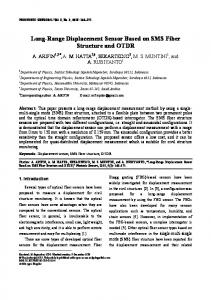
In order to verify the scaling factor map that is related to the data accuracy of the TVDS, a marker related to the the data data accuracy accuracy of the the TVDS, TVDS, aa marker marker In order to verify the scaling factor map that is related plate with a thirteen of 50 mm-diameter markers was installed in front of a camera as shown in 50 50 mm-diameter markers was was installed in front a camera as shown Figurein 5, plate with withaathirteen thirteenofof mm-diameter markers installed in of front of a camera asinshown Figure 5, and the SF1 and SF2 values obtained from the size of marker and the scaling factor map, and the5,SFand obtained the size of marker the scaling map, respectively, Figure theSFSF 1 and SF 2 valuesfrom obtained from the sizeand of marker and factor the scaling factor map, 1 and 2 values respectively, were compared. The markers at both ends of the right and left sides were located 50 mm were compared. markersThe at both ends theends rightofand left sides were located mm behind respectively, wereThe compared. markers at of both the right and left sides were 50 located 50 mm behind from the front markers, and for the experiment, the distance between the camera and the from thefrom frontthe markers, and for the experiment, the distance camera the andcamera the marker behind front markers, and for the experiment, thebetween distancethe between and was the marker was increased by 930 mm, up to 930–3720 mm, and the angle between the camera and the increased byincreased 930 mm, up and the mm, angleand between the camera marker marker was by to 930930–3720 mm, up mm, to 930–3720 the angle betweenand thethe camera andplate the marker plate was increased by 10°, up to 0°–60°. The distance and the angle are the variables to affect was increased by increased 10◦ , up toby 0◦ –60 . The distanceThe and the angle variables affect the marker plate was 10°,◦ up to 0°–60°. distance andare thethe angle are thetovariables toimage affect the image distortion, which make difficult to estimate the actual size of marker using the SF2 obtained distortion, which make difficult estimatetothe actual the sizeactual of marker using the using SF2 obtained from the the image distortion, which maketodifficult estimate size of marker the SF2 obtained from the scaling factor map. scaling map. from thefactor scaling factor map.

Figure Scaling factor validation test ausing a 50-mm-diameter marker and a Figure 5. 5. Scaling factor mapmap validation test using 50-mm-diameter marker plate and plate a commercial Figure 5. Scaling factor map validation test using a 50-mm-diameter marker plate and a commercial commercial camera. camera. camera.

Figure 66 shows shows agraph graph thatcompares compares thedifference difference betweenthe the SF 1 andSF SF2 values values atat Figure Figure 6 shows a a graph that that compares the the difference between between the SF SF11 and and SF22 values at distance = 930 mm, angle = 0, and focal length = 45 mm when the error was approximately 0.36%, and distance = 930 mm, angle = 0, and focal length = mm when the error was approximately 0.36%, and distance = 930 mm, angle = 0, and focal length = 45 mm when the error was approximately 0.36%, and thediameter diameter difference difference of the marker was 0.09 mm. These results imply that thethe image distortion was the markerwas was 0.09 mm. These results imply image distortion the diameter difference of the marker 0.09 mm. These results imply thatthat the image distortion was resolved through the the scaling factor map despite thethe short distance. Figure 7 is7aisgraph showing the was resolved through scaling factor map despite short distance. Figure a graph showing resolved through the scaling factor map despite the short distance. Figure 7 is a graph showing the maximum error of SF 2 SF according to the distance and and the angle, and it canitbe seen that the error in the the maximum the distance the angle, bethat seen that thein error 2 according maximum errorerror of SFof 2 according to thetodistance and the angle, and itand can becan seen the error the distance was low, but it increased greatly with an increase in the angle. When the angle was constant, distance was low, but it increased greatly with an increase in the angle. When the angle was constant,

Sensors 2016, 16, 2085

9 of 17

in the distance was low, but it increased greatly with an increase in the angle. When the angle was Sensors 2016, 16, 2085 9 of 17 constant, the difference in diameter with the actual marker with an increase in the distance ranged thetodifference diameter with the marker withgoverned an increase thedistance. distance ranged fromdistance from 0.03 0.11 mm.inThis indicates thatactual the error is not byinthe When the 0.03 to 0.11 mm. This indicates that the error is not governed by the distance. When the distance was was constant, however, the diameter difference with the actual marker ranged from 1.41 to 1.47 mm, constant, however, the diameter difference with the actual marker ranged from 1.41 to 1.47 mm, showing a larger difference compared to the distance. The results of the marker plate test showed showing a larger difference compared to the distance. The results of the marker plate test showed that thethat image distortion caused by by thetheangle thecamera camera the object is significantly the image distortion caused anglebetween between the andand the object planeplane is significantly effect oneffect the on data accuracy, and the proposed scaling factor has the limitation that compensation for the data accuracy, and the proposed scaling factor has the limitation that compensation for ◦ the distorted is necessary when theangle angle is larger 30°. on these results, the angle the distorted imageimage is necessary when the largerthan than 30Based . Based on these results, the angle the camera andstructure the structure was reducedto toless less than than 10° to to reduce the error due due to betweenbetween the camera and the was reduced 10◦ininorder order reduce the error external factors. externaltofactors.

Figure Figure 6. Comparison ofofthe factors calculated the marker and the scaling 6. Comparison the scaling scaling factors calculated by theby marker and the scaling factor map, factor respectively. map, respectively.

Figure 7. Maximum scaling factorerror error between between SFSF 1 and SF2 in with thewith distance the Figure 7. Maximum scaling factor SFaccordance theand distance and 1 and 2 in accordance angle. the angle.

3. Experimental Test Set-Up A three-story scaled model test was conducted using a shake table (QuanserShake Table II, Quanser Consulting Inc., Markham, ON, Canada) in order to measure the dynamic displacement

Sensors 2016, 16, 2085

10 of 17

3. Experimental Test Set-Up Sensors 2016, 16, 2085

10 of 17 A three-story scaled model test was conducted using a shake table (QuanserShake Table II, Quanser Consulting Inc., Markham, ON, Canada) in order to measure the dynamic displacement through the the proposed proposedTVDS. TVDS.The Thedynamic dynamicdisplacement displacement scaled model measured using through of of thethe scaled model waswas measured using the the TVDS and LDS. The displacement data obtained from the LDS were used as reference data to TVDS and LDS. The displacement data obtained from the LDS were used as reference data to verify verify the displacement data reliability of the Figure TVDS. 8Figure shows the of details of themodel scaledand model the displacement data reliability of the TVDS. shows8the details the scaled the and the shake table excitation experiment. shake table excitation experiment.

Figure Dimensions of of the the scaled scaled model model and and experimental experimental set-up set-up of of scaled Figure 8. 8. Dimensions scaled model model white white noise noise excitation test using shake table (unit: mm). excitation test using shake table.

Because the proposed TVDS employs a camera and extracts the shape of the structure by the image convex hull optimization to measure the displacement of the scaled model, the reliability of the event event of of out-of-plane out-of-plane behavior. behavior. The displacement data the displacement data will decrease in the camera despite despite the the out-of-plane out-of-plane behavior behavior if homography homography transformation transformation could be extracted using a camera is applied and the camera is installed at an angle to the moving plane of the structure. However, the convex hull hulloptimization optimizationused usedininthis thisstudy studyhas has a limitation extracting points required image convex a limitation in in extracting thethe points required for for the transformation. Hence, an X-shape brace was installed in a longitudinal direction of the scaled the transformation. Hence, an X-shape brace was installed in a longitudinal direction of the prevent out-of-plane behavior the scaled The and member and properties materials model totoprevent thethe out-of-plane behavior of theofscaled model. model. The member materials properties of model the scaled model are summarized of the scaled are summarized in Table 1. in Table 1. Table 1. 1. Member properties of the scaled scaled model. model. Member Member Column Column Girder Girder Brace Brace Slab Slab

Material Size (mm) Material Section Section Size (mm) SS400 SS400 Acrylic Acrylic

5 ×55× 5 4 ×46× 6 4×6 4×6 5t 5t

The weight of the mass plate of each floor was approximately 2.0 kg, and the total mass of the scaled model was approximately 9.08 kg. To facilitate the detection of the dynamic characteristics of the structure from the obtained displacement data, a load was applied to the specimen with a

Sensors 2016, 16, 2085

Sensors 2016, 16, 2085

11 of 17

11 of 17

The weight of the mass plate of each floor was approximately 2.0 kg, and the total mass of the scaled model was approximately 9.08 kg. To facilitate the detection of the dynamic characteristics of the structure from the obtained displacement data, a load was applied to the specimen with a 50-Hz-bandwidth white noise, as shown in Figure 9. White noise was generated using MATLAB, 50-Hz-bandwidth white noise, as shown in Figure 9. White noise was generated using MATLAB, and and the white noise generated up to 0–50 Hz included a total of 513 frequency components at the white noise generated up to 0–50 Hz included a total of 513 frequency components at 0.0977 Hz 0.0977intervals. Hz intervals. The TVDS extracted feature points bybyoptimizing areaof ofthe theimage image convex obtained The TVDS extracted feature points optimizing the the area convex hullhull obtained on on the first frame, with the right side of the scaled model as the ROI. The distance between the camera the first frame, with the right side of the scaled model as the ROI. The distance between the camera ◦ . From these and the model waswas 1300 mm, the focal 18 mm, mm,and andthe theangle angle was andscaled the scaled model 1300 mm, the focallength length was was 18 was 3°. 3From these external environments, the calculated scaling factor in the center position imagewas wasfound foundto be external environments, the calculated scaling factor in the center position ofof thethe image be 0.8840 mm/pixel. image of the scaled model was captured with the Nikonatcamera 0.8840tomm/pixel. The imageThe of the scaled model was captured with the Nikon camera 1920 ×at1080 1920 × 1080 (2.0 megapixels) and 60 fps. (2.0 megapixels) and 60 fps.

Figure 9. 50 Hz-bandwidth white noise. (a) Time domain acceleration data; (b) Frequency domain Figure 9. 50 Hz-bandwidth white noise. (a) Time domain acceleration data; (b) Frequency domain representation data.data. representation

Test Results Discussion 4. Test4.Results and and Discussion This section describes analysis thereliability reliability of of the data obtained This section describes thethe analysis ofofthe the dynamic dynamicdisplacement displacement data obtained fromTVDS. the TVDS. displacement databased basedon onvision vision were with the the reference from the The The displacement data weredirectly directlycompared compared with reference data of LDS. In addition, the natural frequency and mode shape of the scaled model were extracted data of LDS. In addition, the natural frequency and mode shape of the scaled model were extracted using the obtained displacement data, and a comparison with the analytical values was conducted using the obtained displacement data, and a comparison with the analytical values was conducted using a commercial program named “MIDAS-Gen”. using a commercial program named “MIDAS-Gen”. 4.1. Comparison of Dynamic Displacement Data

4.1. Comparison of Dynamic Displacement Data

A direct comparison of the dynamic displacement data between LDS and TVDS was performed

Aindirect the dynamic displacement datadata between LDSfrom andthe TVDS was performed order comparison to analyze theofreliability of dynamic displacement obtained TVDS. Figure 10 in order to analyze the reliability of dynamic displacement data obtained fromfrom the the TVDS. Figure shows a time-displacement graph that compares the displacement data obtained TVDS and 10 shows a time-displacement graph that compares the displacement data obtained from the TVDS and LDS of the scaled model to which white noise was applied. With respect to the size and period of the data, the displacement data of the scaled model obtained from the TVDS was in good agreement with the displacement data obtained from the LDS. In addition, it was found that the TVDS can precisely measure not only a relatively large displacement of 40 to 70 mm in the structure at the time of white noise excitation, but also a relatively small displacement of less than 4 mm occurring during free

LDS of the scaled model to which white noise was applied. With respect to the size and period of the data, the displacement data of the scaled model obtained from the TVDS was in good agreement with the displacement data obtained from the LDS. In addition, it was found that the TVDS can precisely measure only a relatively large displacement of 40 to 70 mm in the structure at the time of12white Sensors 2016,not 16, 2085 of 17 noise excitation, but also a relatively small displacement of less than 4 mm occurring during free vibration after excitation. Figure 10b shows that the graph obtained by expanding the displacement vibration after excitation. Figure 10bfloor. shows graph expanding the displacement data measured at 3 to 5 s on the 1st Asthat can the be seen in obtained the Figureby10b, some differences occurred data measured at 3 to 5 s on the 1st floor. As can be seen in the Figure 10b, some differences in the maximum and minimum values between the two measured data, but the vibration occurred period of in thescaled maximum minimum the modeland matched well.values between the two measured data, but the vibration period of the scaled model matched well.

Figure Comparisonofofdynamic dynamicdisplacement displacement data between VDS according to floor the Figure10. 10. Comparison data between VDS andand LDSLDS according to the floor level. (a) 1st floor; (b) detail comparison of the 1st floor; (c) 2nd floor; (d) 3rd floor; (e) peak level. (a) 1st floor; (b) detail comparison of the 1st floor; (c) 2nd floor; (d) (e) peak displacement displacementerror. error.

Usingthe thescaling scalingfactor factormap mapcalculated calculatedfrom fromthe thefocal focallength, length,angle, angle,and anddistance distanceof ofthe thescaled scaled Using model and the camera, the pixel coordinates could be converted to physical coordinates. The scaling model and the camera, the pixel coordinates could be converted to physical coordinates. The scaling factorof ofthe thecentral centralportion portionofofthe theimage imagewas was0.8840 0.8840mm/pixel, mm/pixel, and and that that at at the the end end corner corner of ofthe the factor image was 1.1508 mm/pixel. In addition, as one pixel was divided into five pixels (five-subpixel level) image was 1.1508 mm/pixel. In addition, as one pixel was divided into five pixels (five-subpixel in theinoriginal image when processing thethe image data, the 0.1768 to to level) the original image when processing image data, theresolution resolutionofofthe the TVDS TVDS was was 0.1768 0.2302 mm/pixel. If the subpixel level will be increased, the resolution of the TVDS will be lowered, 0.2302 mm/pixel. If the subpixel level will be increased, the resolution of the TVDS will be lowered, and thus, the accuracy of the sensor can be enhanced. However, there are disadvantages to increasing the subpixel level because the time needed for extracting displacement data from the image will increase and the pixel information of the original image can be distorted. Accordingly, an appropriately

Sensors 2016, 16, 2085

13 of 17

adjusted subpixel level is necessary. Although the one by one comparison of the two displacement data is a good way to reveal the true difference between both data, it is difficult to directly compare the two data sets because of the different sampling rates of the two sensors. Hence, the differences in the peak displacements of LDS and TVDS were compared, and the peak error represented the peak difference between them was calculated from Equation (6). Figure 10e shows the peak error between LDS and TVDS in accordance with the floor level. The maximum peak error is error is 7.16% on the 1st floor, 5.97% on the 2nd floor, and 6.06% on the 3rd floor, and the absolute mean value of peak error is 3.36% on the 1st floor, 3.70% on the 2nd floor, and 2.69% on the 3rd floor. The aforementioned experiment, as shown in Figure 10b,e, revealed that sufficient sensor resolution can be secured for the displacement data obtained using the TVDS, even when compared to the LDS with a 0.01 mm resolution: Peak error (%) =

TVDS − LDS × 100% LDS

(6)

where, TVDS and LDS are the peak displacement obtained each measuring methods. To quantitatively analyze the reliability of the displacement data obtained from the TVDS, it was numerically compared with the LDS through root mean square (RMS) analysis, and the results are summarized in Table 2. The RMS difference between the LDS and the TVDS was 0.22% on the 1st floor, 2.85% on the 2nd floor, and 1.12% on the 3rd floor. Although the biggest error occurred on the 2nd floor, the numerical error between the two data did not exceed 3%. This indicates that even though there is no natural or artificial marker that can be referred to as a target in the structure, the use of the proposed TVDS makes it possible to acquire the dynamic displacement with high reliability. Table 2. Displacement data reliability results on the scaled-model excitation test.

Story 1 2 3

RMS (mm) LDS

TVDS

8.0810 9.7498 10.9949

8.0988 10.0356 11.1191

Error 0.22% 2.85% 1.12%

4.2. Dynamic Characteristics Extracted from VDS If the dynamic characteristics of the structure can be extracted using the obtained displacement data, they can be used for system identification or damage assessment, and therefore, the analysis of the reliability of the obtained dynamic characteristics is important for verifying sensor performance. The dynamic characteristics of the structure, such as the mode shape and natural frequency, were extracted by converting the time domain displacement data to frequency domain data. Figure 11 shows a graph that compares the natural frequencies obtained by the LDS and TVDS. Both sensors yielded 3.27 Hz as the primary natural frequency, and the value of the amplitude was also similar. The secondary natural frequency was not obtained noticeably in the second or third floor data, but it was 10.95 Hz in the displacement data of the first floor. The reason for the failure to obtain more than the third natural frequencies definitely in both the TVDS and the LDS from the second and third displacement data is that it is easy to obtain the data of a low-frequency domain owing to the characteristics of the displacement data, and the sampling rates of 1.67 ms (TVDS) and 1 ms (LDS) are too high for obtaining the natural frequencies of more than 10 Hz of the scaled model. To verify the accuracy of the dynamic characteristics obtained from the displacement data, the natural frequencies were compared after modeling the scale model using the numerical analysis program MIDAS-Gen. The results are summarized in Table 3. The error between the natural frequency obtained using the numerical analysis model and that obtained based on the experiment results was less than 1%. Further, in the experiment, both the LDS and TVDS failed to obtain the third natural frequencies. It can be seen that the TVDS can extract the primary and secondary natural frequencies

Sensors 2016, 16, 2085

14 of 17

Sensors 2016, 16, 2085 of 17 results was less than 1%. Further, in the experiment, both the LDS and TVDS failed to obtain the14third natural frequencies. It can be seen that the TVDS can extract the primary and secondary natural frequencies almost precisely and thus secure a performance to LDS that in of this the LDS in this almost precisely and thus secure a performance identical to identical that of the experiment. experiment. The comparison of the experiment and analytical data revealed that the natural The comparison of the experiment and analytical data revealed that the natural frequency of the scaled Sensors 2016, 16, 2085model obtained by the numerical analysis model was higher than 14 of 17that of the frequency of the scaled model obtained by the numerical analysis model was higher than that of the experiment results. This is experiment results. is because theinstiffness of theboth beam-to-column connection of thethird actual scaled results was This less 1%. Further, the experiment, thethe LDSactual and TVDS failedmodel to obtain the because the stiffness ofthan the beam-to-column connection of scaled was idealized as a model wasnatural idealized asnumerical a rigid in numerical analysis model. frequencies. It canconnection beanalysis seen thatmodel. thethe TVDS can extract the primary and secondary natural rigid connection in the

frequencies almost precisely and thus secure a performance identical to that of the LDS in this experiment. The comparison of the experiment and analytical data revealed that the natural frequency of the scaled model obtained by the numerical analysis model was higher than that of the experiment results. This is because the stiffness of the beam-to-column connection of the actual scaled model was idealized as a rigid connection in the numerical analysis model.

Figure 11. 11. Comparison Comparison of of natural natural frequencies frequencies obtained obtained from from the the TVDS TVDS and and LDS LDS according according to to the the floor floor Figure level. (a) (a) 1st 1st floor; floor; (b) (b) 2nd 2nd floor; floor; (c) (c) 3rd 3rd floor. level. floor. Figure 11. Comparison of natural frequencies obtained from the TVDS and LDS according to the floor level. (a) 1st floor; (b) 2nd floor; (c) 3rd floor.

Table 3. Experimental and analytical natural frequencies of the scaled model. Table Table 3. Experimental and analytical natural frequencies of the scaled model.

of Mode Analytical AnalyticalModel Model(Hz) (Hz) No. No. of Mode No. of Mode

1 2 3

1

1

2

2

3

3

Analytical Model (Hz)

3.31 3.31 3.31 11.08 11.08 11.08 17.57 17.57 17.57

Test Result (Hz) Test Result (Hz)

Test Result (Hz)

LDS TVDS LDS TVDS TVDS 3.27 (0.82%) 3.27 3.27 (0.82%) 3.27 (0.82%) (0.82%) 3.27 (0.82%) 3.27 (0.82%) 10.95 (0.94%) 10.95 (0.94%) 10.95 (0.94%) 10.95 (0.94%) 10.95 (0.94%) 10.95 (0.94%) - LDS

Figure 12 shows a comparison of the numerical and experimental mode shapes of the scale

12 of of thethe numerical andand experimental modemode shapes of the of scale Figuremodel. 12 shows showsa acomparison comparison numerical experimental shapes themodel. scale model.

Figure 12.Figure Comparison of the mode shapes themodel. scaled model. 12. Comparison of analytical the analyticaland andexperimental experimental mode shapes of the of scaled

The experimental mode shapes obtained by both the LDS and the TVDS were similar, and the results only differed slightly from the mode shape obtained numerically. The reason for the difference is that the connection stiffness of the numerical model and that of the actual scaled model are different; Figure 12. Comparison of the analytical and experimental mode shapes of the scaled model. this is similar to the case of the differences in the natural frequency. It was experimentally confirmed that the use of the proposed TVDS makes it possible to precisely obtain the mode shape and natural

Sensors 2016, 16, 2085

15 of 17

frequency of the structure, and the accuracy of the obtained data was verified through comparison with the analysis results. 5. Conclusions In this study, a target-less vision-based displacement sensor (TVDS) was developed to measure the displacement data of the structures without any target such as an artificial or a natural marker in the image. The core technologies of the TVDS are the image convex hull optimization algorithm for extracting the feature points without the artificial markers attached to the structure or natural markers such as a bolt hole in the structure, and a scaling factor map that converts the pixel coordinates of the extracted feature point to physical coordinates using the external environment between the camera and the structures. The reliability of the displacement data obtained by the TVDS was verified experimentally through an excitation test for a three-story scaled model, and through a marker plate test. The study results are summarized as follows: (1)

(2)

(3)

In the TVDS, the scaling factor map is used to convert the pixel coordinates of the feature point obtained from the image convex hull optimization algorithm to physical coordinates. Unlike the existing scaling factor obtained from the diameter of the marker, the scaling factor map can be calculated from the distance between the camera and the marker, the angle, and the focal length. The factor is calculated in accordance with the pixel coordinates of the feature point on the image plane. In the marker plate experiment designed for estimating the diameter of a 50-mm-diameter marker, the error depending on the distance was up to 2%, and that depending on the angle was up to 6%. That is, the error of the estimation by the proposed TVDS was caused to a greater extent by the angle than by the distance. Hence, it is necessary to measure the angle between the camera and the target and set it within 10◦ at the maximum in actual applications. The white-noise excitation test of the three-story scaled model revealed that as the TVDS does not require artificial or natural markers, it can provide the displacement data of three floors from one image. In addition, the difference between the RMS values of the displacement data obtained by the TVDS and the reference data LDS was 0.22%–2.85%, and therefore, it was experimentally verified that the TVDS can perform multiple extraction of highly reliable displacement data with a single camera. To determine if TVDS is a suitable sensor for monitoring a structure, the dynamic characteristics of the structure, such as the mode shape and natural frequency, were extracted using the displacement data obtained by the TVDS. The primary natural frequency values of the scale model obtained by the TVDS and the LDS were identical (3.27 Hz), showing only a 0.82% difference from the primary natural frequency obtained using the numerical analysis model (3.31 Hz). In addition, the mode shape obtained by the TVDS was very similar to the experimental mode shape obtained by the LDS and the analytical mode shape obtained based on the numerical analysis results. In other words, as the displacement data and the dynamic behavior of a structure can be precisely measured through the proposed TVDS, the TVDS is considered a suitable sensor for monitoring a building structure.

The proposed TVDS was shown to be capable of measuring the displacement of the desired part of the structures precisely by using the image convex hull optimization algorithm and scaling factor map. It could also measure the dynamic characteristics of the structure, such as the mode shape or natural frequency. Therefore, as the use of the TVDS makes it possible to obtain the displacement data of a structure without using any target, which is required by the existing vision-based displacement sensor (VDS), the TVDS is expected to become more widely used in the structure monitoring field in the future. Acknowledgments: This research was supported by Basic Science Research Program through a National Research Foundation of Korea (NRF) grant funded by the Ministry of Science, ICT & Future Planning (2014R1A1A1037787) and the Yonsei University Future-leading Research Initiative of 2016 (2016-22-0063).

Sensors 2016, 16, 2085

16 of 17

Author Contributions: Insub Choi and JunHee Kim provided the main idea for this study; Insub Choi and JunHee Kim conceived and designed the experiments; Insub Choi and Donghyun Kim performed the experiments; JunHee Kim supervised the project. All authors contributed to the analysis and conclusion. Conflicts of Interest: The authors declare no conflict of interest.

References 1. 2. 3. 4. 5. 6. 7. 8. 9. 10. 11. 12. 13. 14.

15. 16. 17. 18. 19. 20. 21. 22.

Choi, I.; Kim, J.H.; You, Y.-C. Effect of cyclic loading on composite behavior of insulated concrete sandwich wall panels with GFRP shear connectors. Compos. Part B Eng. 2016, 96, 7–19. [CrossRef] Kim, J.H.; You, Y.-C. Composite Behavior of a Novel Insulated Concrete Sandwich Wall Panel Reinforced with GFRP Shear Grids: Effects of Insulation Types. Materials 2015, 8, 899–913. [CrossRef] Choi, I.; Kim, J.; Kim, H.-R. Composite Behavior of Insulated Concrete Sandwich Wall Panels Subjected to Wind Pressure and Suction. Materials 2015, 8, 1264–1282. [CrossRef] Xu, Z.; Lu, X.; Guan, H.; Han, B.; Ren, A. Seismic damage simulation in urban areas based on a high-fidelity structural model and a physics engine. Nat. Hazards 2014, 71, 1679–1693. [CrossRef] Haber, R.; Unbehauen, H. Structure identification of nonlinear dynamic systems—A survey on input/output approaches. Automatica 1990, 26, 651–677. [CrossRef] Moaveni, B.; He, X.; Conte, J.P.; Restrepo, J.I.; Panagiotou, M. System Identification Study of a 7-Story Full-Scale Building Slice Tested on the UCSD-NEES Shake Table. J. Struct. Eng. 2011, 137, 705–717. [CrossRef] Furukawa, T.; Ito, M.; Izawa, K.; Noori, M.N. System Identification of Base-Isolated Building using Seismic Response Data. J. Eng. Mech. 2005, 131, 268–275. [CrossRef] Kim, J.H.; Ghaboussi, J.; Elnashai, A.S. Hysteretic mechanical–informational modeling of bolted steel frame connections. Eng. Struct. 2012, 45, 1–11. [CrossRef] Kim, J.H.; Ghaboussi, J.; Elnashai, A.S. Mechanical and informational modeling of steel beam-to-column connections. Eng. Struct. 2010, 32, 449–458. [CrossRef] Park, K.-T.; Kim, S.-H.; Park, H.-S.; Lee, K.-W. The determination of bridge displacement using measured acceleration. Eng. Struct. 2005, 27, 371–378. [CrossRef] Park, H.S.; Kim, J.M.; Choi, S.W.; Kim, Y. A Wireless Laser Displacement Sensor Node for Structural Health Monitoring. Sensors 2013, 13, 13204–13216. [CrossRef] [PubMed] Casciati, F.; Fuggini, C. Engineering vibration monitoring by GPS: Long duration records. Earthq. Eng. Eng. Vib. 2009, 8, 459–467. [CrossRef] Sensors, Vision, Measurement and Microscope. Available online: http://www.keyence.com/ (accessed on 21 July 2016). Abdel-Aziz, Y.I.; Karara, H.M.; Hauck, M. Direct Linear Transformation from Comparator Coordinates into Object Space Coordinates in Close-Range Photogrammetry. Photogramm. Eng. Remote Sens. 2015, 81, 103–107. [CrossRef] Jain, J.; Jain, A. A Displacement Measurement and Its Application in Interframe Image Coding. IEEE Trans. Commun. 1981, 29, 1799–1808. [CrossRef] Hatze, H. High-precision three-dimensional photogrammetric calibration and object space reconstruction using a modified DLT-approach. J. Biomech. 1988, 21, 533–538. [CrossRef] Chen, L. An investigation on the accuracy of three-dimensional space reconstruction using the direct linear transformation technique. J. Biomech. 1994, 27, 493–500. [CrossRef] Olaszek, P. Investigation of the dynamic characteristic of bridge structures using a computer vision method. Measurement 1999, 25, 227–236. [CrossRef] Kim, S.-W.; Jeon, B.-G.; Kim, N.-S.; Park, J.-C. Vision-based monitoring system for evaluating cable tensile forces on a cable-stayed bridge. Struct. Heal. Monit. 2013, 12, 440–456. [CrossRef] Feng, D.; Feng, M.Q. Model Updating of Railway Bridge Using In Situ Dynamic Displacement Measurement under Trainloads. J. Bridg. Eng. 2015, 20, 1–12. [CrossRef] Song, Y.-Z.; Bowen, C.R.; Kim, A.H.; Nassehi, A.; Padget, J.; Gathercole, N. Virtual visual sensors and their application in structural health monitoring. Struct. Heal. Monit. 2014, 13, 251–264. [CrossRef] Nogueira, F.M.A.; Barbosa, F.S.; Barra, L.P.S. Evaluation of structural natural frequencies using image processing. In Proceedings of the International conference on experimental vibration analysis for civil engineering structures, Bordeaux, France, 26–28 October 2005; pp. 359–365.

Sensors 2016, 16, 2085

23. 24. 25.

26. 27. 28. 29. 30. 31. 32. 33. 34. 35. 36. 37. 38.

39. 40. 41. 42.

43. 44.

17 of 17

Lee, J.J.; Shinozuka, M. Real-Time Displacement Measurement of a Flexible Bridge Using Digital Image Processing Techniques. Exp. Mech. 2006, 46, 105–114. [CrossRef] Lee, J.J.; Shinozuka, M. A vision-based system for remote sensing of bridge displacement. NDT E Int. 2006, 39, 425–431. [CrossRef] Ji, Y. A computer vision-based approach for structural displacement measurement. In Proceedings of the Sensors and Smart Structures Technologies for Civil, Mechanical, and Aerospace Systems, San Diego, CA, USA, 7 March 2010; Volume 7647, pp. 76473H-1–76473H-11. Park, J.-W.; Lee, J.-J.; Jung, H.-J.; Myung, H. Vision-based displacement measurement method for high-rise building structures using partitioning approach. NDT E Int. 2010, 43, 642–647. [CrossRef] Lee, J.J.; Ho, H.N.; Lee, J.H. A vision-based dynamic rotational angle measurement system for large civil structures. Sensors 2012, 12, 7326–7336. [CrossRef] [PubMed] Choi, H.-S.; Cheung, J.-H.; Kim, S.-H.; Ahn, J.-H. Structural dynamic displacement vision system using digital image processing. NDT E Int. 2011, 44, 597–608. [CrossRef] Kim, S.W.; Kim, N.S. Multi-point displacement response measurement of civil infrastructures using digital image processing. Procedia Eng. 2011, 14, 195–203. [CrossRef] Ho, H.-N.; Lee, J.-H.; Park, Y.-S.; Lee, J.-J. A Synchronized Multipoint Vision-Based System for Displacement Measurement of Civil Infrastructures. Sci. World J. 2012, 2012, 1–9. [CrossRef] [PubMed] Ri, S.; Numayama, T.; Saka, M.; Nanbara, K.; Kobayashi, D. Noncontact Deflection Distribution Measurement for Large-Scale Structures by Advanced Image Processing Technique. Mater. Trans. 2012, 53, 323–329. [CrossRef] Casciati, F.; Casciati, S.; Wu, L.J. Vision-Based Sensing in Dynamic Tests. Key Eng. Mater. 2013, 569–570, 767–774. [CrossRef] Jurjo, D.L.B.R.; Magluta, C.; Roitman, N.; Batista Gonçalves, P. Analysis of the structural behavior of a membrane using digital image processing. Mech. Syst. Signal Process. 2015, 54, 394–404. [CrossRef] Zhan, D.; Yu, L.; Xiao, J.; Chen, T. Multi-camera and structured-light vision system (MSVS) for dynamic high-accuracy 3D measurements of railway tunnels. Sensors 2015, 15, 8664–8684. [CrossRef] [PubMed] Zhang, D.; Guo, J.; Lei, X.; Zhu, C. A High-Speed Vision-Based Sensor for Dynamic Vibration Analysis Using Fast Motion Extraction Algorithms. Sensors 2016, 16. [CrossRef] [PubMed] Park, H.S.; Kim, J.Y.; Kim, J.G.; Choi, S.W.; Kim, Y. A new position measurement system using a motion-capture camera for wind tunnel tests. Sensors 2013, 13, 12329–12344. [CrossRef] [PubMed] Oh, B.K.; Hwang, J.W.; Kim, Y.; Cho, T.; Park, H.S. Vision-based system identification technique for building structures using a motion capture system. J. Sound Vib. 2015, 356, 72–85. [CrossRef] Casciati, F.; Wu, L.J. Structural Monitoring Through Acquisition of Images. In Mechanics and Model-Based Control of Advanced Engineering Systems; Belyaev, K.A., Irschik, H., Krommer, M., Eds.; Springer: Vienna, Austria, 2014; pp. 67–74. Fukuda, Y.; Feng, M.Q.; Narita, Y.; Tanaka, T. Vision-Based Displacement Sensor for Monitoring Dynamic Response Using Robust Object Search Algorithm. IEEE Sens. J. 2013, 13, 4725–4732. [CrossRef] Feng, M.Q.; Fukuda, Y.; Feng, D.; Mizuta, M. Nontarget Vision Sensor for Remote Measurement of Bridge Dynamic Response. J. Bridg. Eng. 2015, 20, 4015023. [CrossRef] Feng, D.; Feng, M.Q.; Ozer, E.; Fukuda, Y. A vision-based sensor for noncontact structural displacement measurement. Sensors 2015, 15, 16557–16575. [CrossRef] [PubMed] Xu, Y.; Brownjohn, J.; Hester, D.; Koo, K.Y. Dynamic displacement measurement of a long span bridge using vision-based system. In Proceedings of the 8th European Workshop On Structural Health Monitoring (EWSHM 2016), Bilbao, Spain, 5–8 July 2016. Barber, C.B.; Dobkin, D.P.; Huhdanpaa, H. The quickhull algorithm for convex hulls. ACM Trans. Math. Softw. 1996, 22, 469–483. [CrossRef] Jayaram, M.A.; Fleyeh, H. Convex Hulls in Image Processing: A Scoping Review. Am. J. Intell. Syst. 2016, 6, 48–58. © 2016 by the authors; licensee MDPI, Basel, Switzerland. This article is an open access article distributed under the terms and conditions of the Creative Commons Attribution (CC-BY) license (http://creativecommons.org/licenses/by/4.0/).