A Theory of Lowest-Price Guarantees
Noah Lim C T Bauer College of Business University of Houston
Teck-Hua Ho1 Haas School of Business University of California at Berkeley
June 6, 2008
1
We thank Ed Blair, Colin Camerer, Ganesh Iyer, John Morgan, Rafael Robb, Niladri Syam and
Miguel Villas-Boas for helpful comments. We are grateful to Sung Ham, Lori Luo and Caroline Nguyen for research assistance. This research is partially supported by the Wharton-Singapore Management University Research Center. Direct correspondence to any author. Lim:
[email protected], Bauer College of Business, University of Houston, Houston, TX 77204. Ho:
[email protected], Haas School of Business, University of California at Berkeley, Berkeley, CA 94720.
A Theory of Lowest-Price Guarantees Noah Lim and Teck-Hua Ho
Abstract
Retailers often offer lowest-price guarantees (LPGs) to support their lowest-price claims. This paper argues that when firms decide whether to offer LPGs, it is important to consider how LPGs can affect customer behavior and in turn the firms’ payoffs. We present an experimental field survey that demonstrates two implications on customer behavior when LPGs are offered: First, LPGs induce consumers to postpone price search till after purchase. Second, relative to the case where there are no LPGs, there are additional customer goodwill effects depending on whether firms post higher or lower prices. Specifically, firms gain goodwill if consumers discover after purchase that the price they had paid is indeed lower; conversely, they suffer goodwill losses if consumers find out that the price they had paid is higher. We incorporate these behavioral implications into a model of price competition where firms offer LPGs. Our model shows that the presence of goodwill effects exerts downward pressure on prices and can result in lower equilibrium prices and less profit compared to a regime without LPGs, even if LPGs lower the level of customer search. These results hold both when customer goodwill is modeled as exogenous or endogenous to the difference in posted prices.
1
1
Introduction
Retailers often offer lowest-price guarantees (LPGs) to support their lowest-price claims. Such guarantees usually promise to refund customers the difference between the firm’s price and the lowest price in the market within a stipulated time (ranging from 24 hours to 45 days) after the purchase. The question of whether firms should offer LPGs has been an area of substantial interest among researchers. The earliest work argue that LPGs can help firms sustain collusive prices because they communicate to rival firms that it will be difficult to gain market share by undercutting prices. This is because customers, who are assumed to search prices before purchase, will not switch firms because they can always invoke the LPG to obtain the lowest price (Salop, 1986, Doyle 1988). Png and Hirshleifer (1987) extends the rationale for offering LPGs by showing that when not all customers search prices, LPGs serve as a price discriminatory device that allows retailers to charge higher prices to those customers who do not search. Recently, two papers (Moorthy and Winter 2006, Moorthy and Zhang 2006) refined the arguments for offering LPGs by showing that not all competing firms should offer LPGs. If rival firms have appreciable differences in costs or service levels, LPGs should only be offered only by the firm with the lower cost or service level, and LPGs serve as a signaling device to the uninformed customers about that firm’s lower price. These papers also presented some empirical evidence to support the theoretical result that LPGs are offered mostly by stores with lower price profiles in the market. We note however that these models share a common prediction with earlier work in that LPGs still have the effect of raising prices - the store that offers the LPG charges a higher price relative to the case where it could not offer the guarantee. There have also been research which argue that in some cases, firms might not want to offer LPGs at all. Hviid and Shaffer (1999) show that if customers incur hassle costs of obtaining refunds, prices will be competitive rather than monopolistic because firms have the incentive to steal market share through lowering price by less than the amount of hassle cost. Chen et. al. (2001) show that if introducing LPGs encourage some consumers to undertake price search before purchase, prices and profits will be lower than if LPGs were not offered. While these papers underline the importance of studying what happens to consumers when LPGs are offered and how they can affect firm’s payoffs and pricing
2 decisions, they did not provide empirical evidence to bolster their assumptions about customer behavior. This paper contributes to the literature on LPGs in the following ways: We contend that when firms evaluate whether to offer LPGs, it is important to examine how introducing LPGs to the market can change customer behavior and perceptions, and consequently, the firms’ payoffs. Our paper builds on the extant behavioral research on LPGs and proposes that there are two changes to customer behavior when firms offer LPGs: first, LPGs induces customers to shift from pre-purchase to post-purchase price search. Second, there are positive and negative goodwill effects (relative to the case when no LPGs are offered) depending on whether the lowest price claims are true. These two hypotheses are supported by an experimental field survey. We then develop a model of price competition with LPGs that incorporates these behavioral findings into the payoff functions of the firms. In the model, we formulate the goodwill effects in two ways: 1) as a term that is independent of the difference in the posted prices of the competing firms, and 2) as a function of the price differential. The model shows that the switch to post-purchase search raises prices, while the goodwill effects intensify price competition. If the goodwill effects are sufficiently strong, average prices can be lower even if the proportion of customers who search and receive the lowest prices in the market is lower in the LPG regime. We also posit that two variants of LPGs, Automatic Price Protection (APP) and price-beating guarantees, may promote fiercer price competition. The paper proceeds as follows: Section 2 develops the hypotheses on the implications of offering LPGs on customer behavior, followed by the design and results of the experimental field survey. In section 3, we present a model of a LPG duopoly that explicitly incorporates the behavioral findings into the firm’s profit functions. We first specify customer goodwill as independent of the difference in the posted prices of the firms. We then characterize the solution to the model and compare the equilibrium prices to a benchmark model without LPGs. Section 4 extends the specification of customer goodwill to include the case where it is also a function of the price difference, and Section 5 concludes.
3
2
Implications of LPGs on Customers
In this section, we examine and test the implications of the introduction of LPGs by competitive firms on consumer behavior and perceptions. To begin, we note that consumer psychologists have studied how consumers interpret LPGs and how the presence of LPGs affects the price image of the firm and customer search behavior, prior to the consumer’s purchase decision. The chief findings from this literature are that consumers believe that firms offering LPGs will have lower prices than those which do not (Jain and Srivastava 2000), and that LPGs lower pre-purchase search levels and increase in-store purchase incidence (Srivastava and Lurie 2001). LPGs are thus perceived by consumers to be devices that support the lowest-price claims of retailers - consumers expect to pay the lowest price and do not expect to invoke the guarantee and claim a refund. Moreover, this perception is strengthened when consumers believe that firms will pay a penalty for posting prices that are higher than the competition (Srivastava and Lurie 2004). We extend consumer research on LPGs by focusing on how LPGs affect customer’s post-purchase attitudes and behavior. First, LPGs give consumers the option to postpone price search till after purchase without any financial penalty. Hence, we would expect the levels of pre-purchase search to be lower (consistent with Srivastava and Lurie 2001) and post-purchase search to be higher when LPGs are offered in the market. Formally, the first hypothesis is: H1: The level of pre-purchase search will be lower and post-purchase search will be higher when LPGs are offered by firms. Next, since customers believe firms offering LPGs have the lowest prices and trust the firm’s claims enough to make an immediate purchase (Srivastava and Lurie 2001), one would expect customer goodwill to be strengthened and reinforced when prices are found to be indeed the lowest. On the other hand, if the price of the firm offering the LPG were found to be higher, there would be goodwill losses because consumers feel that the firms are dishonest about their low price claims, and that they were misled into stopping price search and making the purchase. This goodwill loss can be exacerbated if customers do not have the opportunity to redeem the refund due to reasons such as hassle costs (Hviid and Shaffer 1999) or having missed the stipulated window of opportunity for
4 claiming the refund. Of course, even if consumers receive price-matching refunds, firms can lose goodwill if the redemption process is unpleasant1 . Also, while we believe that there can also be goodwill effects when there are no LPGs (e.g., the lower-priced firms gain customer goodwill from customers who search), we hypothesize that they are not as strong as when firms offer LPGs, because consumers’ expectations that a firm will have the lowest price are not as high if LPGs were not offered to underpin low-price claims. Formally, the second hypothesis is: H2a: If customers discover after purchase that the competitor’s price is higher, the positive goodwill effects are stronger when LPGs are offered. H2b: If customers discover after purchase that the competitor’s price is lower, the adverse goodwill effects are stronger when LPGs are offered. The two hypotheses above have not been studied by marketing researchers. As mentioned above, the extant behavioral research on LPGs have focused on pre-purchase search and have not examined the link between LPGs and the shifts from pre-purchase to post-purchase search. While Srivastava and Lurie (2004) alluded to the possibility that firms might pay a penalty if their low-price claims are not confirmed, they did not directly study the consequences when consumers actually discover competitor’s posted prices; that is, whether there will be goodwill losses when competitor’s prices are lower or goodwill gains otherwise. Moreover, we focus on whether there are differences in customer goodwill when there are LPGs compared to the case where no LPGs are offered. This is critical because the firms’ payoffs in the LPG regime will be different from the payoffs in the no-LPG regime only if there are differences in the goodwill effects across the pricing regimes.
2.1
Design and Procedure of Field Survey
We conducted an experimental field survey to test the two hypotheses. The survey was administered during “Homecoming Day” at a public research university in a major US 1
Conversely, we are open to exceptions where firms can prevent goodwill losses if they manage the
redemption process extremely well, such as offering an Automatic Price Protection (APP) program, which we discuss later in this paper. Moreover, the fact that some firms offer refunds that are greater than the actual differential in posted prices can be seen as a way to mitigate against goodwill losses.
5 metropolitan area. Respondents were approached by student assistants recruited by the researchers, and the assistants were unaware of the hypotheses that were being studied. Respondents were told that the purpose of the survey is to find out how consumers behave in different shopping scenarios. They were asked to indicate responses that most accurately describe their typical shopping behavior. A total of 173 respondents participated in the study. The average age of the respondents is in the 26-30 range and 61% of the respondents are female. In the design, we manipulated two factors: a) whether LPGs were offered by the two firms described in the questionnaire (Yes or No), and b) whether the posted price of the store where they had made the purchase (named JJ Electronics), was higher or lower compared to the price at the competitor store (named KK City). Note that in our study, LPGs were either offered by both firms in the market or not at all. This is different from prior research, where only a single firm offers an LPG. Moreover, in the condition where LPGs were offered and the price of the competitor was lower, we studied two scenarios: whether consumers received a price-matching refund (Yes or No). Together, the design yields the following five conditions (see also Table 1): S1: No LPGs offered, Competitor firm has Higher Price S2: No LPGs offered, Competitor firm has Lower Price S3: LPGs offered, Competitor firm has Higher Price S4: LPGs offered, Competitor firm has Lower Price, Refund Received S5: LPGs offered, Competitor firm has Lower Price, Refund Not Received The survey procedure can be summarized as follows (please refer to Appendix 1 for full details of the procedure and the questions we asked the respondents): Respondents were told to imagine that they were shopping for a good digital camera and that there were two comparable stores, JJ Electronics and KK City, in their local area. In the conditions where LPGs were offered in the market (S3, S4 and S5), respondents were given the additional information that “Each of these two stores also claim to have the best prices in town and offer the following guarantee: if you find a lower price for the identical product in another store within 45 days of your purchase, the store will refund you the difference in prices”. Respondents were next told that they had decided to visit JJ Electronics and saw a
6 camera that met their criteria (the posted price of the camera is 479 dollars). They were then asked how likely they are to search prices at KK City. Afterwards, they were told to imagine that they had decided to purchase the camera at JJ Electronics. They were then asked to indicate their likelihood of post-purchase price search. Next, respondents were told that a few days after the purchase, they saw a newspaper advertisement by KK City, listing the same camera which they had bought. The advertised price at KK City was either 429 or 529 dollars. In the conditions where LPGS were offered and KK City had a lower price (S4 and S5), respondents either obtained the price-matching refund or did not. Respondents in all the treatment conditions were then directed to answer three questions on their post-purchase satisfaction, likelihood of future purchase at JJ Electronics, and their image of JJ Electronics. These questions were meant to capture different facets of customer goodwill.
2.2
Results
The mean responses to the questions respondents were asked are presented in Table 1. The results of the hypothesis tests are as follows: Hypothesis 1 - Changes in Search Behavior. We first examine if there are differences in customers’ price-search behavior when LPGs are offered. First, the data shows that pre-purchase search is lower when firms offer LPGs. When LPGs are offered (S3, S4 and S5 pooled), the mean response to the question on the likelihood of pre-purchase search is 4.03, whereas it is 5.96 (t=7.49, p=0.000) when there are no LPGs (S1 and S2 pooled). This result confirms previous findings that LPGs decreases pre-purchase search. Next, the results show that customers are more likely to look out for the other store’s price after purchase when LPGs were offered (Means 4.95 (S3, S4 and S5 pooled)> 4.10 (S1 and S2 pooled), t=2.58, p=0.006). Together, these findings show that H1 is supported - LPGs do induce in-store customers make purchases immediately and postpone price search till after purchase. Hypothesis 2 - Additional Goodwill Effects in the Presence of LPGs. The responses from the three questions that captures customer goodwill were collapsed to form a single measure (Cronbach’s α=0.91). To begin, we performed the following three manipulation
7 checks: First, two-sided t-tests confirm that when LPGs are not offered, goodwill is indeed higher when the competitor’s price is found to be higher (Means 5.39 (S1) > 3.69 (S2), t=7.16, p=0.000). Similarly, when LPGs are offered, goodwill is higher when the competitor’s price is higher (Means 5.95 (S3) > 3.08 (S4 and S5 pooled), t=12.78, p=0.000). Third, the results confirm that when LPGs are offered and the competitor’s price is lower, customer goodwill is higher when customers received a refund (Means 3.75 (S4) > 2.39 (S5), t=4.34, p=0.001). Next, we test Hypotheses 2A and 2B, which predicts that there are differential effects on customer goodwill when LPGs are offered versus when they are not. First, as predicted by H2a, when the price of the competitor’s firm (KK City) is higher, we find that customer goodwill is higher when LPGs are offered (Means 5.95 (S3) > 5.39 (S1), t=2.56, p=0.013). Second, when the price of competitor firm is higher, customer goodwill is indeed lower when LPGs are offered (Means 3.08 (S4 and S5 pooled) < 3.69 (S2), t=-2.46, p=0.0156), consistent with the prediction of H2b. This is true especially when customers did not receive the price-matching refund (M 2.39 (S5) < 3.69 (S2), t=-4.92, p=0.000). Overall, the results suggest that the effects of post-purchase customer goodwill are amplified if firms offer LPGs: the firm experiences a stronger rise in goodwill when customers confirm that its price is indeed lower; conversely, the firm suffers a relative decline in goodwill when its price is found to be higher, especially when customers do not have the opportunity to redeem the price-matching refund.
3
Model
The results of the field survey demonstrate that 1) the intensity of post-purchase search increases and that 2) positive and negative goodwill effects are stronger when firms introduce LPGs. Next, we formulate a model that incorporates these findings into the firms’ payoffs. Our purpose is to examine how these changes in customer behavior will affect equilibrium prices in a competitive setting. Consider a symmetric duopoly where the firms, denoted by i and j, set prices in a non-differentiated product market. Each firm claims that it has the lowest price and guarantees a refund of the difference if it charges a higher price. Firms have zero marginal costs and set prices Pi , Pj ∈ [0, 1]. Each
8 firm has a customer base of 1 so that the total market size is 2.2 Every customer has a willingness to pay of 1 and purchases a unit of the product before price search. We assume that a fraction α of the firm’s customers will undertake post-purchase price search and receive a price-matching refund if its posted price is higher. Note that α represents a subset of all those customers who search prices after purchase. This fraction is analogous to the fraction of consumers who engage in pre-purchase search when firms do not offer LPGs, as both these segments of consumers pay the lowest price in the market. If the firm’s posted price is higher so that the lowest-price claims are untrue, it suffers a goodwill loss of L(Pi , Pj ) > 0, which is the net present value of the potential loss in future profits. If the firm’s lowest price claim is found to be true, the firm gains customer goodwill. These are cases where a firm’s posted price is either lower than or equal to the competitor’s, and the gains are denoted G(Pi , Pj ) > 0 and G (Pi , Pj ) > 0 respectively. We would expect a firm’s lowest-price claim to be more credibly established if its price is lower rather than identical to its competitor, so G(Pi , Pj ) ≥ G (Pi , Pj ) in general. The payoffs for firm i can thus be written as: ⎧ ⎪ P + G(Pi , Pj ) ⎪ ⎪ ⎨ i
Πi (Pi , Pj ) = ⎪ Pi + G (Pi , Pj )
if Pi < Pj if Pi = Pj
⎪ ⎪ ⎩ αP + (1 − α)P − L(P , P ) if P > P j i i j i j
(3.1)
In equation (2.1) above, the first line is the sum of the profit and gain in goodwill when the firm charges a lower price. The second line denotes the profit and goodwill gain when prices are identical. The first two terms of the last line represent the profit adjusted for giving out LPG refunds when the firm charges a higher price, while the last term denotes the loss in goodwill. In order to study whether introducing LPGs lead to higher or lower prices, we compare our model to a benchmark model without LPGs. This benchmark model is a standard model of price competition (e.g., Narasimhan 1988) which assumes that a fraction of α ˆ consumers search prices before purchase. These customers always purchase from the firm with the lowest price. The payoffs for firm i in the benchmark model is specified as 2
The results for the case where firms have unequal customer bases are qualitatively similar to those
presented in this paper.
9 follows:
Πbi
⎧ ⎪ (1 + α ˆ ) · Pi ⎪ ⎪ ⎨
= ⎪ Pi
⎪ ⎪ ⎩ (1 − α ˆ ) · Pi
if Pi < Pj if Pi = Pj
(3.2)
if Pi > Pj
Comparing equations (2.1) and (2.2), we note the following differences in assumptions. First, the timing of search moves from before the purchase in the benchmark model to after purchase when there are LPGs. In comparing the equilibrium prices of benchmark and LPG models, we believe it is important to allow for α ˆ ≥ α, because there is evidence
that the post-purchase redemption rate of price-matching refunds (a subset of those consumers who search after purchase) is low (Moorthy and Zhang 2006)3 . Second, we do not model goodwill effects explicitly in the benchmark model. As we mentioned earlier, this does not mean that there are no ex-post goodwill effects when LPGs are not offered. Rather, we interpret the goodwill effects G(Pi , Pj ), G (Pi , Pj ) and L(Pi , Pj ) in the LPG model as the incremental changes in goodwill gains or losses relative to the no-LPG regime. These incremental goodwill changes were demonstrated in the field survey in the previous section. To begin our analysis, we characterize the equilibrium prices in the benchmark model in the following proposition (the proofs for all the propositions in this paper are in the Appendix): Proposition 1 : For α ˆ ∈ (0, 1), there exists a symmetric mixed-strategy Nash equilib-
rium with the following strategy profile4 : 3
There is very little data on redemption rates available to researchers. Moorthy and Zhang (2006)
relies on survey data from 46 North American retailers. Among those retailers who responded, most of the redemption rates are below 10%, with the maximum at only 25%. While this information is useful, we note that retailers have the incentive to under-report redemption rates, since high rates of redemption are incongruent with their low-price claims. 4 If α ˆ = 1, equilibrium prices are Bertrand. If α ˆ = 0, the Pareto-dominant equilibrium is the monopolist price pair (1, 1).
10
⎧ ⎪ 0 ⎪ ⎪ ⎨
F b (Pi ) = ⎪ where Pmb =
1−α ˆ . 1+α ˆ
1 2α ˆ
⎪ ⎪ ⎩ 1
1+α ˆ−
1−α ˆ Pi
if Pi ∈ [0, Pmb );
if Pi ∈ [Pmb , 1);
(3.3)
if Pi = 1;
The expected price is: E(Pi ) =
1−α ˆ 1+α ˆ ln 2ˆ α 1−α ˆ
(3.4)
The above proposition shows the well-known result that prices decline in the intensity of pre-purchase search α ˆ . We will use the results in Proposition 1 to evaluate the relative competitiveness of prices in markets with LPGs.
3.1
Exogenous Goodwill
In this section, we solve the LPG model assuming that customer goodwill depends solely on whether prices are lower or higher, independent of the price differential between the two firms. In general, the magnitude of gains and losses in customer goodwill need not be identical; however, since this does not affect the results qualitatively, we present only the case where G(Pi , Pj ) = L(Pi , Pj ) = γ > 0 and G (Pi , Pj ) = γ0 > 0. In the following propositions, we focus on characterizing the properties of a symmetric mixed-strategy Nash equilibrium for the case where γ > γ0 5 . Proposition 2 For α ∈ (0, 1), there is a symmetric mixed-strategy Nash equilibrium that can be characterized as follows6 : 5 6
If γ = γ0 , the Pareto-dominant equilibrium is the monopolist price pair (1, 1). Note that there is a Bertrand equilibrium if γ + γ0 ≥ (1 − α). If α = 1, prices are Bertrand for
any positive γ. If α = 0 and γ ∈ (0, 12 ), there is a symmetric mixed-strategy Nash equilibrium with the following strategy profile:
⎧ ⎪ ⎪ ⎨ 0 F (Pi ) = 1− ⎪ ⎪ ⎩ 1
1−Pi 2γ
if Pi ∈ [0, Pm ); if Pi ∈ [Pm , 1);
if Pi = 1;
11 Case 1. If γ
0,
> 0, and limα→1 F (0) = 1.
Comparison with Pricing Regime Without LPGs
The LPG model differs from the benchmark model in two significant ways: 1) customers conduct post-purchase instead of pre-purchase search, and 2) it incorporates the additional positive or negative goodwill that are due to the introduction of lowest-price claims where Pm = 1 − 2γ. The expected price is 1 − γ.
If α = 0 and γ ∈ [ 12 , 1), then there is a mass point at Pi = 0, and the mixed-strategy equilibrium is : ⎧ 1 ⎪ if Pi = 0; ⎪ ⎨ 1 − 2γ 1−P i F (Pi ) = if Pi ∈ (0, 1); 1 − 2γ ⎪ ⎪ ⎩ 1 if Pi = 1;
with an expected price of
1 4γ .
12 backed by LPGs. We proceed to examine the relative competitiveness of LPG model by analyzing the incremental effect of each of these changes. In comparing the two pricing regimes, we will also allow α to be lower than α ˆ. Figure 1 shows the effect of a change from pre-purchase to post-purchase search behavior in the absence of customer goodwill (i.e., when γ = γ0 = 0). Note that in the benchmark model, expected prices decline with search intensity α ˆ . In the LPG model, if there are no goodwill effects, a price cut by a firm will not attract customers from the rival firm but will reduce revenue from its own customers. Hence, the effect of the change in search pattern is to raise prices to monopoly levels for all positive values α. When goodwill effects are present equilibrium prices decline with the rate of refund redemption (i.e.,
∂E(Pi ) ∂α
< 0). Figure 2 describes this relationship for 0 < α < 1 and
γ = 0.25 while keeping the level of pre-purchase search in the benchmark model and the post-purchase redemption rate in LPG regimes identical (i.e., α = α ˆ ). More importantly, Figure 2 also shows that equilibrium prices can be higher or lower with LPGs. The following proposition states this result formally (see Appendix for proof): Proposition 3 Assume the fraction of customers who will receive the lowest prices in the market, i.e., α = α ˆ ∈ (0, 1) and γ ∈ (0, 1). Let α ˜ ≈ 0.655 be the solution to the following implicit equation:
1−α 1+α 1 1 + 1 + ln ln(1 − α) α 2 1−α
=0
(3.9)
Case 1: α < α ˜ . LPG regime is more competitive than the benchmark regime if γ > γ ∗ , where γ ∗ is characterized in (3.10). Otherwise, LPG regime is less competitive.
ln( 1+α )−α 1−α γ = 1 2(1 + α ln(1 − α)) ∗
1−α 2
(3.10)
Case 2: α ≥ α ˜ . LPG regime is more competitive than the benchmark regime if γ > γ ∗ ,
where γ ∗ solves the implicit equation (3.11). Otherwise, LPG regime is less competitive.
13
α
2γ ∗ (e 2γ ∗ − 1) = α 1 +
1 1+α ln 2 1−α
(3.11)
The term γ ∗ traces the iso-competitive curve for the two regimes, which is defined as the level of goodwill where expected prices in both regimes are equal (see Figure 3). In the region above the iso-competitive curve, the LPG regime is more competitive, whereas it is less competitive in the region below the curve. This result is interesting as it shows that LPG regime can lead to more competitive prices if the fraction of customers who will receive the lowest prices in the market is identical in both price regimes. The LPG regime may still be more competitive even if the post-purchase redemption rate in the LPG regime is lower than the level of pre-purchase search in the benchmark model. Figure 4 illustrates such an example, where α ˆ = 0.3 and γ = 0.25, and from 0 to 1 (i.e., α varies from 0 to 0.3). Note that as
α α ˆ
α α ˆ
varies
increases, expected prices
decrease and become lower than those of the benchmark model when
α α ˆ
exceeds 0.53.
Hence, the prediction of lower prices if firms offer LPGs in our model does not hinge on an increase in the proportion of customers who search (c.f. Chen et. al. 2001). Finally, since goodwill is central to our model, it is interesting to see how it influences equilibrium prices. Figure 5 shows the effect of customer goodwill γ on equilibrium prices for two levels of α. Equilibrium prices decline linearly in customer goodwill for γ
Pj , firm i’s payoff in an APP duopoly is: ⎧ ⎪ P +γ ⎪ ⎪ ⎨ i
if Pi < Pj
Πi (Pi , Pj ) = ⎪ Pi + γ0 if Pi = Pj ⎪ ⎪ ⎩ P j
(3.12)
if Pi > Pj
It is easy to see that there is a pure-strategy equilibrium at (0,0) when γ > γ0 , when the firm performs searches on behalf of the customers (and hassle costs are absent). It is interesting to note that the APP policy has been discontinued by Tweeter8 . The special case of α = 1, that is, full customer search and redemption after purchase, is also related to the Traveler’s Dilemma (Basu 1994), which can also be interpreted as a type of price-matching game. In this game, the payoffs are identical to those of the APP, except that γ will be subtracted from the firm’s payoffs when the firm’s posted price is higher. This again results in Bertrand pricing for any γ > 0. However, Capra et. al (1999) and Goeree and Holt (2001)) studied Traveler’s Dilemma game experimentally and showed that prices are seldom at Bertrand levels unless γ is large. Specifically, there is an inverse relationship between prices and the level of customer goodwill not predicted by theory. Our main model shows that as long as the limiting condition of α = 1 is slightly relaxed, prices are above Bertrand and also vary inversely with γ. Hence, one possible explanation of the experimental results are that subjects could be making decisions based on beliefs that α is less than one. 7
The survey results show that when customers receive rebates (S4), there is no significant difference
in goodwill in the LPG and no-LPG regimes. Specifically, when there are LPGs and refunds are received (S4), the mean response on customer goodwill is 3.74. When LPGs are not offered, the mean response is 3.69 (S2). The t-stat is 0.23, p-value=0.814. Moreover, the scenario in S4 was that consumers were told that they had to return to the store to receive a refund - customers have to do even less under APP. 8 A check on Tweeter’s website at www.tweeter.com shows that Tweeter has a conventional pricematching guarantee, that is, one where customers have a show proof of a lower price by another store within 30 days of the purchase.
15
3.2
Goodwill Endogenous to Prices
We extend the formulation of customer goodwill to include the case where the magnitude of goodwill effects is also a function of the price differential between the firms. A straightforward way to operationalize this is to assume that customer goodwill varies linearly with the price differential. Specifically, for firm i, we define G(Pi , Pj ) = γ0 + ωG · (Pj − Pi )
and L(Pi , Pj ) = γ0 + ωL · (Pi − Pj ), where ωG > 0 and ωL > 0 represents the constant
marginal gain and loss in customer goodwill (when firms post identical prices, G (Pi , Pj )
is unchanged and equal to γ0 ). The payoffs for firm i is given by:
⎧ ⎪ P + γ0 + ωG · (Pj − Pi ) ⎪ ⎪ ⎨ i
if Pi < Pj
Πi = ⎪ Pi + γ0 if Pi = Pj ⎪ ⎪ ⎩ αPj + (1 − α)Pi − γ0 − ωL · (Pi − Pj ) if Pi > Pj
(3.13)
The solution to the model can delineated into three cases depending on whether ωG > 1 and (1 − α) − ωL > 0. Note that when ωG > 1, the marginal gain in customer goodwill outweighs the loss in revenue from the price cut. This incentive is absent when ωG ≤ 1. If (1 − α) − ωL ≤ 0, the benefit of increased revenue from raising prices is
outweighed by the loss in goodwill. When (1 − α) − ωL > 0, there are cases where the
firm has an incentive to raise prices. The formal solution is characterized in the following proposition (see Appendix for the proof and also Figure 6):
Proposition 4 The symmetric Nash equilibria in each of the three cases are: Case I. If ωG > 1 and (1 − α) − ωL ≤ 0, the equilibrium prices are Bertrand. Case II. When ωG > 1 and (1 − α) − ωL > 0, the solution depends on the relative
magnitude of (1 − α) − ωL and 2γ0 . If (1 − α) − ωL ≤ 2γ0 , prices are Bertrand. If (1 − α) − ωL > 2γ0 , there are multiple equilibria. There are two asymmetric pure-strategy equilibria are (0, 1) and (1, 0) and there is a symmetric mixed-strategy equilibrium where firms choose either 0 or 1. The probability that a firm chooses 1 is is also the expected price of this equilibrium.
1−(α+ωL +2γ0 ) , ωG −(α+ωL +2γ0 )
which
16 Case III. If ωG ≤ 1, the Pareto-dominant equilibrium is the monopolist price pair (1, 1) 9
.
Proposition 4 suggests that if customer goodwill varies linearly with the price differential, equilibrium prices are at either the Bertrand or monopoly levels. The implication we draw is identical similar to the case when goodwill effects are exogenous: to decide if offering LPGs raises prices and profits, it is crucial for firms to measure the size of changes in goodwill effects that arise as a result of introducing LPGs - in Cases I and II, prices are lower when firms offer LPGs (the expected price in the mixed strategy equilibrium in Case II is lower than the benchmark model).
3.2.1
Discussion: Price-Beating Competition
Our model can also be used to examine price-beating competition, i.e., when firms offer to compensate customers an additional percentage of the price differential in addition to the price-matching refund10 . This compensatory amount is commonly fixed at five or ten percent of the price differential. For example, Circuit City currently offers an additional 10% compensation for charging a higher price. Our conjecture is that relative to price-matching, price-beating guarantee may send a stronger signal to customers so that their lowest-price claims become even more credible. This could lead to two effects that intensify price competition. First, more customers would be inclined to redeem the refund as there are larger financial gains (i.e., α increases). Second, goodwill effects can be stronger (i.e., γ0 , ωG and ωL increase). For example, if customers do have not the opportunity to claim the price-beating refunds, their losses would be magnified (since they lose both the refund and the additional compensation). 9
If (1 − α) − ωL ≤ 2γ0 , all symmetric price pairs in [0,1] are Nash equilibria. If (1 − α) − ωL > 2γ0 ,
2γ , 1] the set of equilibria is all symmetric price pairs in [1 − 1−α 10 The LPG model with exogenous goodwill can also represent a form of price-beating competition
where firms offer a lump-sum payment to customers on top of the refund. However, the policy of compensating an additional fraction of the price differential is much more prevalent in practice.
17
4
Conclusion
This paper argues that when firms are evaluating whether to offer LPGs, they must account for the effects of changes in customer behavior as a result of offering LPGs, and how they affect the firms’ payoffs. We use an experimental field survey to demonstrate two examples of such behavioral changes: First, LPGs induce customers to shift from pre-purchase to post-purchase search. Second, there are goodwill effects associated with whether the lowest-price claims of the firms are found to be true. Next, we develop a model of LPG competition that explicitly captures these effects. We compare the equilibrium prices to a benchmark model without LPGs and show that prices can be lower if firms offer LPGs. This result remains valid even if we allow the rate of refund redemption in the LPG regime to be lower than level of pre-purchase search in the noLPG case. The results are also robust to the case where goodwill effects are a function of the difference in the firms’ posted prices. Our model also suggests that policies such as Automatic Price Protection (APP) and price-beating competition may intensify price competition. The implications of this paper are clear: firms should not assume that customer behavior remains static when pricing regimes change. Specifically, to understand the impact of offering LPGs on prices, it is imperative that firms understand factors like that the level of post-purchase search and the fraction of customers who are likely to claim price-matching refunds. Our paper also suggests that firms must examine their policies that that influence the price-matching redemption process, such as the timeframe for redemption, the procedure for claiming refunds, the type of competitor prices and products on which the firm will match prices (e.g., advertised prices, items not on sale, same model number, etc.), as these can influence the direction and the degree of the goodwill effects. These issues have also not been explored by researchers. More research is also needed on the formulating of the goodwill effects, such as how strongly they are affected by differences in posted prices (i.e., values of ωG and ωL ), whether there are asymmetries in the magnitude of positive and negative goodwill changes - for example, the latter effect may be stronger as predicted by Prospect Theory (Kahneman and Tversky 1979), and finally, translating these effects into dollar terms.
18
5
Appendix
5.1
Details of Survey Procedure
In each of the five treatments, respondents were told to imagine that they were shopping for a good digital camera and were willing to pay up to a maximum of 600 dollars. Based on their initial research, they determined that the digital camera must have the following three features: 1) it must be a well-established brand, 2) at least 5 Megapixels, and 3) must have least a 3X optical zoom. Recently, an independent consumer report had rated two stores in their local area, JJ Electronics and KK City, as comparable in terms of customer service, prices and range of products carried in the stores. In the conditions where LPGs were offered in the market (S3, S4 and S5), respondents were given the additional information: “Each of these two stores also claim to have the best prices in town and offer the following guarantee: if you find a lower price for the identical product in another store within 45 days of your purchase, the store will refund you the difference in prices”. Respondents were next told that they had decided to visit JJ Electronics. In the store, they saw the Canon Powershot SD 700 Digital ELPH camera, with 6 Megapixels and a 4X optical zoom (this was one of the best models offered by Canon at the time of the study). The price of the camera is 479 dollars. They were then asked (after a filler question) to indicate the response to the following question: “I am likely to visit KK City to check its price for the same digital camera before deciding where to purchase the camera” (1=Strongly Disagree, 7=Strongly Agree). After answering another filler question, respondents were told that they had decided to purchase the digital camera at JJ Electronics at a price of 479 dollars during that visit. They then answered the following question about their post-purchase search behavior: “After your purchase, how likely are you to look out for the price of the same camera at the other store, KK City? (1=Very Unlikely, 7=Very Likely). Next, respondents were told that a few days later, they saw a newspaper advertisement by the store they did not visit, KK City, listing the price of the same camera they had bought. In the conditions where KK City has a higher price (S1 and S3), respondents saw
19 a price of 529 dollars. In the conditions where KK City’s listed price are lower (S2, S4 and S5), they saw a price of 429 dollars. When LPGS are offered and KK City has a lower price (S4 and S5), respondents read the additional information: In S4, they were told that they “returned to JJ Electronics to ask for a refund for the price difference. After speaking to the store manager and filling out a form, the manager promises to mail you a 50 dollar refund check”. In S5, they were told that “For various reasons, you were unable to return to JJ Electronics to ask for a refund for the price difference”. Respondents were then directed to answer the following three questions that capture different facets of postpurchase customer goodwill: 1) Purchase Satisfaction - “I am satisfied with the decision to purchase the camera at JJ Electronics” (1=Strongly Disagree, 7=Strongly Agree); 2) Likelihood of Future Purchase - “I am likely to return to JJ Electronics to make a similar purchase in the future” (1=Very Unlikely, 7=Very Likely); and 3) Perceptions of Store Image - “My overall image of JJ Electronics is enhanced after this purchase” (1=Not At All, 7=Very Much So). After this, respondents answered one more filler question and some questions that capture demographic variables.
5.2 5.2.1
Proofs of Propositions Proof of Proposition 1
We begin by noting that when α ˆ = 1, prices are Bertrand. When α ˆ = 0, prices are monopolist. Next we consider the case of α ∈ (0, 1). As is well-known from the previous
literature (e.g. Narasimhan 1988), there is no pure-strategy Nash equilibrium, so we look for a symmetric mixed-strategy Nash equilibrium. Define f b (.) and F b (.) to be the
mixing density and cumulative density function (c.d.f.) respectively for either firm over the support [Pmb , 1], where Pmb is the lowest price both firm charge in equilibrium. Denote firm i’s expected profit by E(Πbi ). From equation (2.2), if firm i charges Pi ∈ [Pmb , 1], E(Πbi ) =
1 Pi
((1 + α ˆ )Pi ) · f b (Pj ) dPj +
Pi b Pm
((1 − α ˆ )Pi ) · f b (Pj ) dPj
(5.1)
This yields: E(Πbi ) = Pi (1 + α ˆ ) − 2ˆ αPi F b (Pi )
(5.2)
20 Equating the above with the expected profit when firm i charges 1 (the maximum price) and simplifying, we have F b (Pi ) =
1 1−α ˆ 1+α ˆ− 2ˆ α Pi
(5.3)
Narasimhan (1988) shows that there is no mass point at Pmb so that we have F b (Pmb ) = 0. Solving, we obtain
1−α ˆ 1+α ˆ The expected price for firm i under the mixed-strategy Nash equilibrium is Pmb =
1
E(Pi ) =
b Pm
Pi · f b (Pi ) dPi = 1 −
1 b Pm
F b (Pi ) dPi
(5.4)
(5.5)
This yields E(Pi ) =
5.2.2
1−α ˆ 1+α ˆ ln 2ˆ α 1−α ˆ
(5.6)
Proof of Proposition 2
We consider the case where α ∈ (0, 1). The symmetric mixed-strategy equilibrium depends on whether γ is greater or less than Case 1. γ
0 as long as γ
0, firm i’s expected profit is:
1
E(Πi ) =
Pi
(Pi + γ) · f (Pj ) dPj +
Pi 0+
(αPj + (1 − α)Pi − γ) · f (Pj ) dPj
+F (0)((1 − α)Pi − γ)
(5.16)
This yields E(Πi ) = Pi + γ − 2γF (Pi ) − α
Pi 0+
F (Pj ) dPj
(5.17)
If firm i charges 0, the expected profit is E(Πi ) = (1 − F (0)) · γ + F (0) · γ0
(5.18)
22 Solving for F (.) by equating the two equations and differentiating with respect to Pi , we get F (Pi ) = 1 α
Hence, F (0) =
1 1 α(1−Pi ) + (1 − )e 2γ α α
α
+ (1 − α1 )e 2γ . Note that
∂F (0) ∂α
> 0,
(5.19)
∂F (0) ∂γ
> 0, and limα→1 F (0) = 1.
The expected price is
1
E(Pi ) = F (0) · 0 +
0+
1
Pi · fi (Pi ) dPi = 1 −
0+
Fi (Pi ) dPi
(5.20)
This yields
α 1 − α 2γ 2γ e −1 −1 (5.21) α α −α Note that when γ = 2 ln(1−α) , the expected price in both cases yield an identical value of
E(Pi ) =
α−1 α
−
5.2.3
1 . ln(1−α)
Proof of Proposition 3
We compare the expected price for the benchmark model in equation (2.4) and those of LPGs in equations (2.6) and (2.8) to determine whether LPG is more or less competitive than the benchmark model. Note that when γ =
−α , 2 ln(1−α)
(2.6) and (2.8) give the same
expected price. Define α∗ to be level of post-purchase redemption rate where expected prices in the benchmark and LPG models are identical when γ =
−α . 2 ln(1−α)
α∗ is solved
by equation (2.9), which is obtained by equating expression (2.4) and (2.6) where we set γ=
−α . 2 ln(1−α)
Solving (2.9), we obtain α ˜ = 0.6551. So when α ˜ = 0.6551 and γ˜ = 0.3077,
expected prices are identical in the benchmark and LPG models. When γ < γ˜ , expected price in LPG model is given by (2.6), otherwise it is given by (2.8). For any α, we determine the level of γ that make the two regimes equally competitive. Call this level of goodwill γ ∗ . For α < α ˜, γ ∗ =
1−α 2
1+α ln( 1−α )−α
(2.10). Similarly, for α ≥ α∗ , γ ∗ is solved by the implicit equation 2γ (e 1 2
α 1 + ln
1+α 1−α
, which is
1 2(1+ α ln(1−α)) α ∗ 2γ ∗
− 1) =
, which is (2.11). This iso-competitive curve traces the values of γ ∗ for
all α. Figure 3 shows this iso-competitive curve and the point (˜ α, γ˜ ). Hence, if γ > γ ∗ , the LPG regime is more competitive. If γ ≤ γ ∗ , the LPG regime is less competitive.
23 5.2.4
Proof of Proposition 4
The proofs of Cases I and III are straightforward. We simply check whether the firm has an incentive to deviate by inspecting
∂Πi ∂Pi
for each parametric combination. For Case
III, note that the solution can be characterized by two sub-cases: If (1 − α) − ωL ≤ 2γ0 ,
all symmetric price pairs in [0,1] are Nash equilibria. If (1 − α) − ωL > 2γ0 , the set of equilibria is all symmetric price pairs in [1 −
2γ , 1]. 1−α
For Case II, the symmetric mixed-
strategy equilibrium when (1 − α) − ωL > 2γ0 is obtained by equating the following 2
equations to solve for p, the probability that i charges 1:
E(Πi | Pi = 1) = p · (1 + γ0 ) + (1 − p) · (1 − α − ωL − γ0 )
(5.22)
E(Πi | Pi = 0) = p · (γ0 + ωG ) + (1 − p) · γ0
(5.23)
24
References [1] Basu, K. (1994), ‘The Traveler’s Dilemma: Paradoxes of Rationality in Game Theory’, American Economic Review: Papers and Proceedings, 84 (2), 391-95. [2] Chen, Y., Narasimhan, C. and J. Zhang (2001), ‘Consumer Heterogeneity and Competitive Price-Matching Guarantees’, Marketing Science, 20 (3), 300-314. [3] Capra, M., J.K Goeree, R. Gomez and C. Holt (1999), ‘Anomalous Behavior in a Traveler’s Dilemma?’, American Economic Review, 89 (3), 678-90. [4] Goeree, J. and Holt, C. (2001), ‘Ten Little Treasures of Game Theory, and Ten Intuitive Contradictions’, American Economic Review, 91 (5), 1402-1422 . [5] Gourville, J. and Wu, G. (1996), “Tweeter etc.” Harvard Business School Case 9597-028. [6] Ho, T., N. Lim and C. Camerer (2006a), ‘Modeling the Psychology of Customer and Firm Behavior Using Behavioral Economics’, Journal of Marketing Research, 43 (3), 307-331. [7] Ho, T., N. Lim and C. Camerer (2006b), ‘How Psychological Should Marketing Models Be?’, Journal of Marketing Research, 43 (3), 341-344. [8] Hviid, M. and Shaffer, G. (1999), ’Hassle Costs: The Achilles’ Heel of Price-Matching Guarantees’, Journal of Economics and Management Strategy, 8(4), 489-521. [9] Jain, S. and J. Srivastava, (2000), ‘An Experimental and Theoretical Analysis of Price-Matching Refund Policies’, Journal of Marketing Research, 37, 351-62. [10] Moorthy, S. and R. Winter (2006), ‘Price-Matching Guarantees’, RAND Journal of Economics, 37, 449-465. [11] Moorthy, S. and X. Zhang (2006), ‘Price-Matching by Vertically Differentiated Retailers: Theory and Evidence’, Journal of Marketing Research, 43 (2), 156-167. [12] Narasimhan, C. (1988), ‘Competitive Promotional Strategies’,Journal of Business, 61 (4), 427-449. [13] Salop, S. (1986), ‘Practices that (Credibly) Facilitate Oligopoly Co-ordination’, in J. Stiglitz, and F. Matthewson, eds., New Developments in the Analysis of Market Structure, MIT Press, Cambridge MA, 265-90. [14] Png, I.P.L and D. Hirshleifer (1987),’Price Discrimination through Offers to Match Price’, Journal of Business, 60, 365-383. [15] Srivastava, J. and N. Lurie (2001), ‘A Consumer Perspective on Price-Matching Refund Policies: Effect on Price Perceptions and Search Behavior’, Journal of Consumer Research, 28, 296-307. [16] Srivastava, J. and N. Lurie (2004), ‘Pricing-Matching Guarantees as Signals of Low Store Prices: Survey and Experimental Evidence’, Journal of Retailing, 80 (2), 117128.
Figures and Tables Figure 1 – Effect of Post-Purchase Price Search and Refund Redemption (No Goodwill, γ=γ0=0)
E(Price) 1 0.9 0.8 0.7 0.6
LPG
0.5
BM
0.4 0.3 0.2 0.1
α , αˆ
0 0
0.1 0.2 0.3 0.4 0.5 0.6 0.7 0.8 0.9
1
Figure 2 – Effect of Redemption Rate with Customer Goodwill (γ=0.25)
E(Price) 1 0.9 0.8 0.7 0.6 0.5 0.4
BM LPG
0.3 0.2 0.1 0
α , αˆ 0
0.2
0.4
0.6
0.8
1
Figure 3 – Iso-Competitive Curve (γ∗) for LPG Model
γ∗ 0.4
LPG More Competitive 0.3
0.2
LPG Less Competitive α~ =0.655
0.1
α , αˆ
0 0
0.2
0.4
0.6
0.8
1
Figure 4 – Effect of Reduced Fraction of Customers Paying the Lowest Price with LPGs (αˆ =0.3, γ=0.25)
E(Price) 0.8
0.75
BM
0.7
LPG
0.65
α αˆ
0.6 0
0.2
0.4
0.6
0.8
1
Figure 5 – Effect of Goodwill for α=0.3 and α=0.6
E(Price) 1 0.9 0.8
α=0.3
0.7 0.6
α=0.6
0.5 0.4 0.3 0.2 0.1 0 0
0.2
0.4
0.6
0.8
γ
Figure 6 - Solution to LPG Model with Endogenous Goodwill
ωL ≥1-α
1
I Bertrand
ωG ≤1
If 1-α-ωL≤ 2γ0, Bertrand. If 2γ0