A Theory of Rate-Based Execution - Semantic Scholar

A Theory of Rate-Based Execution* Kevin Jeffay Department of Computer Science University of North Carolina at Chapel Hill Chapel Hill, NC 27599-3175 [email protected] Abstract* We present a task model for the real-time execution of eventdriven tasks in which no a priori characterization of the actual arrival rates of events is known; only the expected arrival rates of events is known. The model, called rate-based execution (RBE), is a generalization of Mok’s sporadic task model [14]. The RBE model is motivated naturally by distributed multimedia and digital signal processing applications. We derive necessary and sufficient conditions for determining the feasibility of an RBE task set and demonstrate that earliest deadline first (EDF) scheduling is an optimal scheduling algorithm for both preemptive and nonpreemptive execution environments, as well as hybrid environments wherein RBE tasks access shared resources. Our analysis of RBE tasks demonstrates a fundamental distinction between deadline based scheduling methods and static priority based methods. We show that for deadlinebased scheduling methods, feasibility is solely a function of the distribution of task deadlines in time. This is contrasted with static priority schedulers where feasibility is a function of the actual arrival rates of work for tasks. Thus whereas the feasibility of static priority schedulers is a function of the periodicity of tasks, the feasibility of deadline schedulers is independent of task arrival processes and hence deadline schedulers are more suitable for use in distributed, eventdriven, real-time systems.

1. Introduction Real-time applications frequently interact with external devices in an event-driven manner. The delivery of a message, or the generation of a hardware interrupt is an event that causes the operating system to schedule a task to respond to the event. In real-time environments, one must provide some form of guarantee that the processing corresponding to an event will complete within d time units of the event’s occurrence. Hard-real-time systems guarantee that every event ei will be processed within di time units of its occurrence. Soft-real-time and firm-real-time systems provide weaker guarantees of timeliness.

Steve Goddard Computer Science & Engineering University of Nebraska — Lincoln Lincoln, NE 68588-0115 [email protected]

ice events at precise, periodic intervals. Events serviced by sporadic tasks have a lower bound on their inter-arrival time, but no upper bound on inter-arrival time. We have found in practice, especially in distributed real-time systems, that the inter-arrival of events is neither periodic nor sporadic. There is, however, usually an expected or average event arrival rate that can be specified. For example, in an Internet video conferencing system, media samples are typically generated precisely periodically. However, after they are transmitted over the network, samples can arrive at the receiver at nearly arbitrary rates. The transmission rate is precise and the average reception rate is precise, but the instantaneous reception rate is potentially unbounded (depending on the amount of buffering in the network). Our goal here is to understand the complexity of directly modeling the rate-based nature of systems such as distributed multimedia systems. We have created a simple model of real-time tasks that execute at well-defined average rates but have no constraints on their instantaneous rate of invocation. Our model of rate-based execution, called RBE, is a generalization of Mok’s sporadic task model in which tasks are expected to execute with an average execution rate of x times every y time units. Our experience designing distributed, event-driven, real-time systems, such as multimedia systems and classes of military signal processing systems, demonstrates that this task model more naturally models the actual implementation and run-time behaviors of these systems [5, 6, 10].

In this work we present necessary and sufficient conditions for determining the feasibility of scheduling an RBE task set on a single processor such that no task misses its deadline. The analysis holds for earliest deadline first (EDF) scheduling which is also shown to be an optimal scheduling algorithm for both preemptive and non-preemptive execution environments, as well as hybrid environments wherein tasks Most real-time models of execution are based on the Liu and access shared memory resources. Layland periodic task model [12] or Mok’s sporadic task model [14]. Periodic tasks are real-time programs that serv- The analysis of EDF scheduling demonstrates a fundamental distinction between deadline based scheduling methods and * Work supported by grants from the National Science Foundation (grants static priority based methods. We show that for deadlineCCR-9510156, CDA-9624662, & CCR-9732916) and the IBM Corpora- based scheduling methods, feasibility is solely a function of tion. the distribution of task deadlines in time and is independent Published in: Proceedings of the 20th IEEE Real-Time Systems Symposium, Phoenix, AZ, December 1999, pages 304-314.

2 of the rate at which tasks are invoked. In contrast, the opposite is true of static priority schedulers. For any static priority scheduler, feasibility is a function of the rate at which tasks are invoked and is independent of the deadlines of the tasks. Said more simply, the feasibility of static priority schedulers is solely a function of the periodicity of tasks, while the feasibility of deadline schedulers is solely a function of the periodicity of the occurrence of a task’s deadlines. Given that it is often the operating system that assigns deadlines to tasks, this means that the feasibility of a static priority scheduler is a function of the behavior of the external environment (i.e. arrival processes) while the feasibility of a deadline driven scheduler is a function of the implementation of the operating system. We believe this is a significant observation as one typically has more control over the implementation of the operating system than they do over the processes external to the system that generate work for the system. Therefore, we conclude that deadline based scheduling methods have a significant and fundamental advantage over priority based methods when there is uncertainty in the rates at which work is generated for a real-time system, such as is the case in virtually all distributed real-time systems. The rest of this paper is organized as follows. Section 2 provides the motivation for considering the RBE task model and describes related work. Section 3 formally presents the RBE task model. Section 4 presents necessary and sufficient conditions for preemptive scheduling, non-preemptive scheduling, and preemptive scheduling with shared resources and demonstrates the optimality of EDF scheduling in each case. Section 5 discusses these results and demonstrates the infeasibility of static priority scheduling. In addition, Section 5 compares RBE to other models of rate-based execution and scheduling such as proportional share resource allocation [2, 13, 15, 19, 21, 22] and server algorithms such as the total bandwidth server [17, 18]. We conclude our presentation of the RBE model with a summary in Section 6.

tions) [8], and tasks may be preempted by interrupt handlers (i.e., realistic device interactions can be modeled) [9]. A set of relations on model parameters that are necessary and sufficient for tasks to execute in real-time are known, and optimal algorithms for scheduling tasks, based on EDF scheduling, have been developed. One practical complexity that arises in applying the existing models of sporadic tasks to actual systems is the fact that the real world does not always meet the assumptions of the model. Consider a task’s minimum inter-invocation time parameter. The formal model assumes that consecutive invocations of a sporadic task are separated by at least p time units for some constant p. Tasks that are invoked in response to events generated by devices such as network interfaces may not satisfy this property. For example, for the simple video conferencing application described in the introduction, when video frames are periodically transmitted across an internetwork, they may be delayed for arbitrary intervals at intermediate nodes and arrive at a conference receiver at a highly irregular rate. One solution to this problem is to simply buffer video frames at the receiver and release them at regular intervals to the application (although this begs the question of how one implements and models the real-time tasks that perform this buffering process). This approach is undesirable because it is difficult and tedious to implement correctly and because buffering inherently increases the acquisition-to-display latency of each video frame (and latency is the primary measure of conference quality).

Our approach is to alter the formal model to account for the fact that there may be significant “jitter” (deviation) in the inter-invocation time of real-time tasks. We develop a characterization of a task that is similar to that of a sporadic task, however, we make no assumptions about the spacing in time of invocations of an RBE task. Instead, we allow one to specify an average execution rate that is desired for a task. In the RBE model, if a task is invoked at time t, the task is scheduled with a deadline for processing that is suffi2. Motivation and Related Work cient to ensure that the task actually makes progress at its The starting point for this work is the model of sporadic specified rate. tasks developed by Mok [14], and later extended by Baruah et al. [4], and Jeffay et al. [9]. A sporadic task is a simple vari- Digital signal processing is another domain in which the ant of a periodic task. Whereas periodic tasks recur at con- RBE task model naturally describes the execution of applicastant intervals, sporadic tasks (as defined by Mok) have a tions. Processing graphs are a standard design aid in the delower bound on their inter-invocation time, which creates an velopment of complex digital signal processing systems. upper bound on their rate of occurrence. The fact that spo- We have found that, even on a single-CPU system with radic tasks may execute at a variable (but bounded) rate periodic input devices, processing graph nodes naturally exemakes them well-suited for supporting event-driven applica- cute in highly aperiodic “spurts” [5, 6]. Moreover, source data often arrives in bursts in distributed implementations of tions. processing graphs. As discussed in Section 5, this fact preBaruah et al. developed the seminal complexity analysis for cludes the efficient modeling of node execution with either determining the feasibility of a sporadic task set [4]. Today, periodic or sporadic task models. the theory of sporadic tasks is general enough to accommodate a model of computation wherein tasks may communi- With respect to previous attempts to explicitly specify a cate via shared memory (i.e., tasks may have critical sec- task’s progress in terms of an execution rate, the RBE task

3 model is most similar to the linear bounded arrival process (LBAP) model as defined and used in the DASH system [1]. In the LBAP model, processes specify a desired execution rate as the number of messages to be processed per second, and the size of a buffer pool used to store bursts of messages that arrive for the process. Our task model generalizes the LBAP model to include a more generic specification of rate and adds an independent response time (relative deadline) parameter to enable more precise real-time control of task executions. Moreover, we analyze the model in more complex environments such as those wherein tasks communicate via shared memory and thus have preemption constraints. A more detailed comparison to other models of rate-based execution is deferred until Section 5.

3. RBE Task Model Here we formally define the concept of rate-based execution and present the RBE task model. A task is a sequential program that is executed repeatedly in response to the occurrence of events. Each instance of the execution of the task is called a job or a task instance. Jobs are made ready for execution, or released, by the occurrence of an event. An event may be externally generated, e.g., a device interrupt, or internally generated, e.g., a message arrival. In all cases, once released, a job must execute to completion before a well-defined deadline. We assume instances of an event type are indistinguishable and occur infinitely often. Thus over the life of a real-time system an infinite number of jobs of each task will be released.

of a task instance and the completion of its execution (i.e., d is the relative deadline of the task), and •

c is the maximum amount of processor time required for any job of task T to execute to completion on a dedicated processor.

The pair (x, y) is referred to as the rate specification of an RBE task. A task with rate specification (x, y) expects to receive and process, on average, x events in every interval of length y. More precisely, jobs of a task are constrained to execute as follows. Let tij be the release of J ij, the jth job of the ith task. We assume throughout that the order of jobs of a task corresponds to the order of event occurrences for the task (i.e., for all i and j, t ij ≤ ti,j+1). Once released, job Jij must complete execution before a deadline Di(j) given by the following recurrence relation: tij + di if 1 ≤ j ≤ xi  Di ( j ) =  max( t + d , D ( j – x ) + y ) if j > xi ij i i i i 

(1)

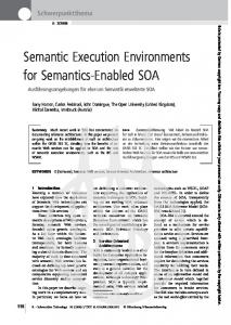
The deadline of a job is the larger of the release time of the job plus its desired deadline or the deadline of the x th previous job plus the y parameter (the averaging interval) of the task. This deadline assignment function confers two important properties on RBE tasks. First, up to x consecutive jobs of a task may contend for the processor with the same deadline and second, for all j, deadlines of jobs Jij and Ji,j+xi of task T i are separated by at least y time units. Without the latter restriction, if a set of jobs of a task were released simultaneously it would be possible to saturate the processor. However, with the restriction, the time at which a task must For a given real-time task, two commonly studied paradigms complete its execution is not wholly dependent on its release of event occurrences are periodic, in which events are gener- time. This is done to bound processor demand. ated every p time units for some constant p, and sporadic, in which events are generated no sooner than every p time units For example, Figure 1 shows the job release times and deadfor some constant p. We consider two fundamental exten- lines for a task T 1 = (x=1, y=2, d=6, c). The downward arsions to these models. First, we make no assumptions about rows in the figure indicate release times for jobs of T 1 . For the relationships between the points in time at which events each job, the interval represented by the open box indicates occur for a task. We assume that events are generated at a the interval of time in which the job must execute to comprecise average rate (e.g., 30 events per second) but that the pletion. (The actual times at which jobs execute are not actual distribution of events in time is arbitrary. Second, we shown.) Figure 1 shows that if jobs of T 1 are released periallow tasks to specify a desired rate of progress in terms of odically, once every 2 time units in this case, then T 1 will the number of events to be processed in an interval of speci- execute as a periodic task with a desired deadline that is different from its period. In particular, if jobs are released perified length. odically then the rate specification of T 1 does not come into Formally, we consider a real-time system to be composed of play in the computation of deadlines. a set of RBE tasks. An RBE task is uniquely characterized Figures 2 and 3 show the effect of job releases that occur at by a four-tuple (x, y, d, c) of integer constants where: the same average rate as before, but where jobs are not re• y is an interval in time, leased periodically. In these figures, three jobs are released • x is the maximum number of executions expected to be simultaneously at time 0, two jobs are released simultanerequested in any interval of length y, ously at time 3, one job is released at time 6, etc. Figure 2 • d is a response time parameter that specifies the maxi- shows the job release times and deadlines for task T 1 = (x=1, y=2, d=6, c). For comparison, Figure 3 shows the effect of mum time that is desired to elapse between the release the same pattern of job releases on a task T 2 = (x=3, y=6,

4

J 1,1

J 1,5 J 1,2

J 1,6

J 1,10

J 1,3

J 1,11

J 1,7 J 1,4

0

2

4

J 1,8 6

processing of each complete media sample, there is no obvious deadline for processing individual fragments of the media sample (other than the deadline for the processing of the complete media sample).

J 1,9

8

10

12

J 1,12 14

16

18

20

22

24

26

28

Figure 1: Release times and deadlines for jobs of T1 = (x=1, y=2, d=6, c). J1,1 J1,2 J1,3 J1,4 J1,5 J1,6 J1,7 J1,8 J1,9 0

2

4

6

8

10

12

14

16

18

20

22

24

26

Figure 2: Bursty release times and deadlines for jobs of T1 = (x=1, y=2, d=6, c). J2,1 J2,2 J2,3 J2,4 J2,5 J2,6 J2,7 J2,8 J2,9 0

2

4

6

8

10

12

14

16

18

20

22

24

Figure 3: Bursty release times and deadlines for jobs of T2 = (x=3, y=6, d=6, c). d=6, c) with the same desired deadline but a different rate specification. Since job releases are not periodic, the actual deadlines of jobs are a function of the rate specification of the task. Note that tasks T1 and T2 will consume the same fraction of the processor and both will complete, on average, one job every two time units. The effect of the different rate specification is two-fold. First, when bursts of events occur, up to three jobs of task T2 may execute with the same deadline. Thus, for example, task T2 might be used to implement the media play-out process in a distributed multimedia system wherein (1) media samples are generated at the precise rate of one sample every six time units at a sender, and (2) each sample is too large to fit into a single network packet and thus is fragmented at the sender into three network packets, which are transmitted one immediately following the other to the receiver. At the receiver, media samples arrive, on average, one sample every two time-units. However, since the sender fragments media samples and transmits the fragments one after the other, it is likely that bursts of three simultaneous (or nearly simultaneous) packet arrivals at the receiver will be common. Moreover, at the receiver, while there is a deadline to complete the

The fundamental problem here is that the arrival rate of inputs at the receiver (3 network packets received every 6 time units), is not the same as the output rate at the receiver (1 media sample displayed every 6 time units). By giving a rate specification of (x=3, y=6), the receiver can effectively process groups of up to three network packets with the same deadline — the deadline for completion of the processing of a media sample. Thus by specifying an execution rate, we avoid the artificial problem of having to assign deadlines to intermediate processing steps. Note that this example is overly simplistic as in practice packet arrivals are discrete events, and hence fundamentally cannot occur “at the same time.” Thus in practice, packets arriving as described above will have deadlines that are separated by at least the minimum inter-arrival time of a pair of packets on the given network transmission medium (e.g., 5 microseconds on a 100BaseT Ethernet). However, the fact that the deadlines for packets arriving in a burst would have slightly offset deadlines has the positive side-effect of ensuring that the operating system will process the packets in arrival order (assuming a deadline-driven scheduler). A task with a rate specification such as T1 in Figure 2, might be used to implement the play-out process in a different multimedia system wherein media samples (such as audio samples) are small enough to fit into a single network packet and thus the packet arrival rate is the same as the sample play-out rate. Here all network packets should have the same relative deadline for completion of processing (e.g., the expected inter-arrival time of packets). The pattern of deadlines in Figure 2 ensures that the play-out application is guaranteed (assuming the workload is feasible) that in the worst case a media sample will be ready for play-out every y time units starting at time 6. The second effect of having different rate specifications for tasks T1 and T2 is that if jobs are not released periodically, jobs of T2 will have a lower guaranteed response time than jobs of T1. Note that there are times at which it is possible for both tasks to have more than xi jobs active simultaneously (e.g., in the interval [0,16] for task T1 and in the interval [3,16] for T2). This is because the rate specification for a task only specifies the rate at which jobs are expected to be released. The actual release rate is completely determined by the environment in which the tasks execute. (In fact, over the entire interval shown in Figures 2 and 3, jobs are released at a slower rate than expected.) Also note that the times when individual jobs complete (and hence whether or not there ever are actually

5

4. Feasibility of RBE Tasks J3,1

Our goal is to determine relations on RBE task parameters that are necessary and sufficient for a set of tasks to be feasible. A set of RBE tasks is feasible if and only if for all job release times tij, and for all Jij, it is possible to execute Jij such that:

J3,2 J3,3 J3,4 J3,5 J3,6 J3,7 J3,8 J3,9 0

2

4

6

8

10

12

14

16

18

20

22

24

1.

Jij commences execution at or after time tij, and

2.

Jij completes execution at or before time Di(j).

Our analysis proceeds by analyzing the demand for the processor created by a set of RBE tasks in an interval of length L. In general the demand for the processor created by any set of real-time tasks is a function of the scheduling discipline in use. Here we limit our consideration to earliest deadline first (EDF) scheduling. We justify this restriction by showing that EDF is an optimal scheduling discipline for RBE tasks. OpFor a final comparison, Figure 4 shows the effect of the job timality here means that an EDF scheduler can guarantee a release times illustrated in Figures 2 and 3 on the task T3 = correct execution to any feasible RBE task set. In Section 5 (x=1, y=2, d=2, c). Task T3 is identical to T1 except with a we discuss alternate scheduling disciplines. smaller desired deadline. Figures 2 and 4 can be used to ilUnder EDF scheduling, the demand for the processor in an lustrate one benefit of decoupling a task’s deadline from its interval is a function of the number of jobs of tasks that have arrival rate and, in particular, the benefit of having a deaddeadlines in the interval. The deadline assignment function line that is greater than the expected inter-job release time. Di(j) decouples the processor demand from the arrival rate of Consider the case where task T1 is used to implement the events and bounds the number of jobs that can have a deadmedia play-out process in a distributed multimedia system line in any given interval. This in turn bounds the processor wherein media samples are generated at the precise rate of demand in any interval. one sample every two time units at the sender. Assume each media sample fits into a network packet and media samples More precisely, the processor demand in an interval [a, b] is are buffered for up to six time units at the receiver prior to the amount of processor time required to be available in [a, b] to ensure that all tasks released prior to time b with deadplay-out to smooth delay-jitter in the network. lines in [a, b] complete in [a, b]. The maximum processor Since samples are expected to be buffered at the receiver, there is little utility to the system in processing samples with demand in an interval [a, b] occurs when Figure 4: Bursty release times and deadlines for jobs of T3 = (x=1, y=2, d=2, c). multiple jobs of a task eligible for execution simultaneously) will depend on the scheduling policy employed. Figures 1-3 should be interpreted as describing a realm of possible execution patterns of tasks.

a deadline that is less than the expected buffer residence time. That is, if a job of T3 completes the processing of a media sample within two units of the sample’s arrival (which is guaranteed to happen if the arrival of media samples is not bursty), then the media sample will reside in a buffer for at least four time units after this processing completes. In contrast, since T1 has a larger desired deadline, one would expect that samples processed by T1 would spend more time waiting to be processed and less time being buffered prior to play-out. Thus the distinction between jobs of T1 and T3 is that the media samples processed by jobs of the former task will likely spend more time waiting to be processed (i.e., “buffered in the run-queue”) and less time in play-out buffers than when processed by jobs of T3. The time between media arrival and play-out will be the same in both cases, however. Thus the desired deadline for task T1 is more appealing in practice as its use will improve the response time for the processing of aperiodic and non-real-time events.

1.

a marks the end of an interval in which the processor was idle (or 0 if the processor is never idle),

2.

the processor is never idle in the interval [a, b], and

3.

as many deadlines as possible occur in [a, b].

To ensure that no job misses a deadline, we must bound the maximum cumulative processor demand of all tasks in all intervals, and verify that the processor has sufficient capacity to satisfy this demand. To begin, we bound the maximum processor demand for an RBE task in the interval [0, L]. Lemma 4.1: For an RBE task T = (x, y, d, c),

 L − d + y (2) ∀L > 0, f   ⋅ xc y   is a least upper bound on the processor demand in the interval [0, L], where a  if a ≥ 0 f (a) =   0 if a < 0

6 Proof: To derive a least upper bound on the amount of processor time required to be available in the interval [0, L], it suffices to consider a set of release times of T that results in the maximum demand for the processor in [0, L]. If t j is the time of the jth release of task T, then clearly the set of release times t j = 0, ∀j > 0, is one such set. Under these release times, x jobs of T have deadlines in [0, d]. After d time units have elapsed, x jobs of T have deadlines every y time units thereafter. Thus the number of jobs with deadlines in the interval [d, L] is

Proof: The necessity of (4) is shown by establishing the contrapositive, i.e., a negative result from evaluating (4) implies that τ is not feasible. To show that τ is not feasible it suffices to demonstrate the existence of a set of task release times for which at least one job of a task in τ misses a deadline. Assume n  l − di + yi  ∃l > 0 : l < ∑ f   ⋅ xi ci . yi  i =1 

 L − d  ⋅ x . Therefore, for all  y  Let tij be the release time of the jth job of task T i. Consider

L > d, the number of jobs of T with deadlines in the interval the set of release times tij = 0, for all i, 1 ≤ i ≤ n, and j > 0. [0, L] is By Lemma 4.1, the least upper bound for the processor deL−d L − d   ⋅ x = 1 +  x +  ⋅x  y   y   

 l − d i + yi   ⋅x c units of proces yi  i i

mand created by task Ti is f 

sor time in the interval of [0, l]. Moreover, from the proof of Lemma 4.1, the set of release times tij = 0, 1 ≤ i ≤ n and j > 0, creates the maximum processor demand possible in (3) the interval [0, l]. Therefore, for τ to be feasible, it is rel − d i + yi  quired that ∑in=1 f  ⋅ x c units of work be available  yi  i i For all L < d, no jobs of T have deadlines in [0, L], hence in [0, l]. However, since the right-hand side of (3) gives the maximum number of n l − di + yi  jobs of T with deadlines in the interval [0, L], for all L > 0. l < ∑ f ⋅x c , yi   i i Finally, as each instance of T requires c units of processor i =1 time to execute to completion, (2) is a least upper bound on the number of units of processor time required to be avail- a job of a task in τ must miss a deadline in [0, l]. Thus able in the interval [0, L] to ensure that no job of T misses there exists a set of release times such that a deadline is missed when (4) does not hold. This proves the contraposia deadline in [0, L]. n tive. Thus, if the task set τ is feasible, (4) must hold. Note that there are an infinite number of sets of job release times that maximize the processor demand of an RBE task To show the sufficiency of (4), it is shown that the preempin the interval [0, L]. For example, it is straightforward to tive EDF scheduling algorithm can schedule all jobs of tasks show that the less pathological set of job release times in τ without any missing a deadline if the tasks satisfy (4). This is shown by contradiction.  j − 1  ⋅ y , ∀j > 0, also maximizes the processor demand tj = Assume that τ satisfies (4) and yet there exists a job of a L−d  =  + 1 ⋅ x  y  − + L d y ⋅x =   y 



x



task in τ that misses a deadline at some point in time when τ is scheduled by the EDF algorithm. Let td be the earliest 4.1 Feasibility under preemptive scheduling point in time at which a deadline is missed and let t0 be the A task set is feasible if and only if there exists a schedule later of: such that no task instance misses its deadline. Thus, if LD • the end of the last interval prior to td in which the procrepresents the total processor demand in an interval of length essor has been idle (or 0 if the processor has never been L, a task set is feasible if and only if L ≥ LD for all L > 0. idle), or The following gives a necessary and sufficient condition for scheduling a set of RBE tasks when preemption is allowed • the latest time prior to td at which a job with deadline after td stops executing prior to td (or time 0 if no such at arbitrary points. job executes prior to td). Theorem 4.2: Let τ = {(x 1, y 1, d1, c1), …, (x n, y n , dn, cn)} By the choice of t 0 , (i) only jobs with deadlines earlier than be a set of RBE tasks. τ will be feasible if and only if: time td execute in the interval [t0, td], (ii) all jobs released n  L − di + yi  prior to time t0 will have completed executing by t0, and (iii) ∀L > 0, L ≥ ∑ f  ⋅ (4) x c  i i yi  the processor is fully used in [t0, td]. It is straightforward to i =1  show that at most where f() is as defined in Lemma 4.1. of task T in the interval [0, L].

7 n

t − t0 − di + yi   ⋅ xi yi

∑  d i =1

Corollary 4.3: EDF is an optimal preemptive scheduling algorithm for sets of RBE tasks.

job of tasks in τ can have deadlines in the interval [t0, td] Proof: Theorem 4.2 has established that independent of the scheduling policy in use, condition (4) is necessary for fea[3], and hence sibility. Moreover, Theorem 4.2 also establishes that (4) is n  td − t0 − di + yi  ⋅ x c sufficient for ensuring that no job will ever miss a deadline ∑   i i y when scheduled by the EDF algorithm. Since (4) is necesi i =1 sary for feasibility and sufficient for a correct execution unis the least upper bound on the units of processor time re- der the EDF algorithm, the EDF algorithm EDF is an optiquired to be available in the interval [t0, td] to ensure that no mal scheduling algorithm for sets of RBE tasks n job misses a deadline in [t0, td] when τ is scheduled under the 4.2 Feasibility under non-preemptive schedEDF algorithm. uling Let ε be the amount of processor time consumed by tasks in We now present necessary and sufficient conditions for τ in the interval [t0, td] when scheduled by the EDF algoevaluating the feasibility of RBE task sets under nonrithm. It follows that preemptive, work-conserving scheduling algorithms (i.e., n the class of scheduling algorithms that schedule non td − t0 − di + yi  ⋅ x c ≥ ε . ∑   i i yi preemptively without inserting idle time in the schedule). i =1 We leave open the problem of deciding feasibility under nonSince the processor is fully used in the interval [t0, td] and work-conserving, non-preemptive scheduling. since a deadline is missed at time t d , it follows that the amount of processor time consumed by τ in [t0, td] when Theorem 4.4: Let τ = {(x 1, y 1, d1, c1), …, (x n, y n , dn, cn)} scheduled by the EDF algorithm is greater than the processor be a set of RBE tasks sorted in non-decreasing order by d time available in [t0, td]. Since the processor time available parameter (i.e., for any pair of tasks Ti and T j, if i > j, then di ≥ dj). τ will be feasible under non-preemptive scheduling in [t0, td] is td – t0, we have if and only if n n  td − t0 − di + yi  ⋅ x c L − di + yi  ∑   i i ≥ ε > t d – t 0 . ∀L > 0, L ≥ f ⋅x c y (6) i i =1 y   i i

∑ i =1

i

However this contradicts our assumption that τ satisfies and equation (4). Hence if τ satisfies equation (4) then no release ∀i, 1 < i ≤ n; ∀L, d1 < L < di : i −1 of a task in τ misses a deadline when τ is scheduled by the  L − 1 − dj + yj  L ≥ ci + f (7)  ⋅ x jcj EDF algorithm. It follows that satisfying (4) is a sufficient yj   j =1 condition for feasibility. Thus, (4) is a necessary and sufficient condition for the feasibility of an RBE task set. n where f() is as defined in Lemma 4.1. If the cumulative processor utilization for an RBE task set is The proofs of this theorem and the following corollary are strictly less than one (i.e., ∑in=1 xyi ci i < 1) then condition (4) contained in the full version of this paper [11]. However, it can be evaluated efficiently (in pseudo-polynomial time) should be noted that they are straightforward extensions of using techniques developed by Baruah et al. [3]. Moreover, the proofs of Theorems 3.2, 3.4 and Corollary 3.4 in [8] for for the special case of di = y i, for all T i in τ , the evaluation non-preemptive scheduling of sporadic tasks. In addition, the of (4) reduces to the polynomial-time feasibility condition optimality of non-preemptive EDF scheduling demonstrated in [8] also holds for RBE tasks. [9] n Corollary 4.5: With respect to the class of nonxi ⋅ ci ≤ 1. (5) preemptive work-conserving schedulers, non-preemptive yi i =1 EDF is an optimal scheduling algorithm for RBE tasks [11]. Equation (5) computes processor utilization for the task set 4.3 Feasibility under preemptive Scheduling τ and is a generalization of the EDF feasibility condition for with shared resources periodic tasks with deadlines equal to their period given by We now consider the case when tasks perform operations on Liu and Layland [12]. shared memory resources. Shared memory resources are seriFinally, note that the proof of the necessity of (4) in Theo- ally reusable but must be accessed in a mutually exclusive rem 4.2 is independent of the scheduling policy in use. This manner. Our model of computation is based on that preallows us to conclude that EDF is an optimal scheduling sented in [8]. algorithm for RBE tasks.

∑

∑

8 Access to a set of m shared resources {R 1, R 2 , …, Rm}, is modeled by specifying the computation requirement of task Ti as a set of ni phases {(cij, Cij, rij) | 1 ≤ j ≤ ni} where:

L ≥ Cik +

i −1

 L − 1 − dj + yj   ⋅ x j ⋅ Ej yj 

∑ f  j =1

(9)

where: c ij is the minimum computational cost: the minimum th • f() is as defined in Lemma 4.1, amount of processor time required to execute the j phase of Ti to completion on a dedicated processor. • δ rik = min ( d j ∃l, 1 ≤ l ≤ n j , rjl = rik ) , 1≤ j ≤ n • C ij is the maximum computational cost: the maximum E j = ∑ln=1 C jl , and amount of processor time required to execute the jth • phase of Ti to completion on a dedicated processor. if k = 1  0 Sik =  k −1 • rij is the resource requirement: the resource (if any) that • ∑ j =1 cij if 1 < k ≤ ni is required during the jth phase of T i. If rij = k, 1 ≤ k ≤ m , then the jth phase of T i requires exclusive access to The feasibility conditions are similar to (and in fact a generresource Rk. If rij = 0 then the jth phase of T i requires no alization of) those for non-preemptive scheduling. The pashared resources. rameter Ei represents the maximum cost of a job of task T i The execution of each job of task T i is partitioned into a and replaces the ci term in conditions (6) and (7) of Theorem sequence of n i disjoint phases. A phase is a contiguous se- 4.4. Condition (9) now applies to only a resource requesting quence of statements that together either require exclusive phase of a job of task T i rather than to the job as a whole. access to a single shared resource, or require no shared re- Because of this, the range of L in (9) is more restricted than scheduling. The sources. In the latter case, the jth phase of T i imposes no in the single phase case of non-preemptive th range is more restricted since the k phase of a job of task T i mutual exclusion constraints on the execution of other cannot start until all previous phases of the job have termitasks. If a phase of a task requires a resource then the comnated, and thus the earliest time phase k can be scheduled is putational cost of the phase represents only the cost of using th S time units after the start the job. For the k phase of a ik the required resource and not the cost (if any) of acquiring or job, the range of intervals of length L in which one must releasing the resource. Note that since different tasks may perform different operations on a resource, it is reasonable to compute the achievable processor demand will be shorter assume that phases of tasks that access the same resource than in the single phase case by the sum of the minimum have varying computational costs. A minimum cost of zero costs of phases 1 through k – 1. Moreover, no demand of phases of Ti other than k appear in (9). Finally, note that for indicates that a phase of a task is optional. the special case where each task in τ consists of only a sinWe assume that in principal tasks are preemptable at arbi- gle phase, the scheduling problem reduces to simple nontrary points. The requirement of exclusive access to re- preemptive scheduling and conditions (8) and (9) reduce to sources places two restrictions on the preemption and execu- the feasibility conditions of Theorem 4.4. tion of tasks. For all task i and k, if rij = rkl and rij, rkl ≠ 0, then (i) the jth phase of a job of T i may neither preempt the The proofs of Theorem 4.6 and the following corollary are lth phase of a job of Tk, nor (ii) execute while the lth phase of contained in the full version of this paper [11]. It is again the case that they are straightforward extensions of the Tk is preempted. proofs in the original paper ([8]) for scheduling sporadic Consider a set of RBE tasks τ = {T1, T2, …, Tn}, where T i = tasks that share a set of shared memory resources. (x i, yi, di, {(c ij, C ij, rij) | 1 ≤ j ≤ ni}), that share a set of resources {R 1, R 2 , …, Rm}. Let δ i represent the deadline pa- A generalized EDF scheduling algorithm was introduced in rameter of the “shortest” task that uses resource R i. That is, [8] to schedule sporadic tasks that share a set of resources. δ i = min (dj | rj = i). The following theorem establishes This algorithm was shown to be optimal for sporadic tasks. 1≤ j ≤ n It is also optimal for RBE tasks that share a set of shared memory resources. necessary and sufficient conditions for feasibility. •

j

Theorem 4.6: Let τ be a set of RBE tasks, sorted in nondecreasing order by d parameter, that share a set of serially reusable resources {R1, R2, …, Rm}. τ will be feasible under work-conserving scheduling if and only if ∀L > 0, L ≥

n

∑ f  i =1

L − di + yi  ⋅x ⋅E yi  i i

and ∀i, 1 < i ≤ n; ∀k, 1 ≤ k ≤ ni ∧ rik ≠ 0; ∀L, δ rik

(8)

Corollary 4.7: With respect to the class of workconserving schedulers, generalized EDF is an optimal scheduling algorithm for RBE task sets that share a set of serially reusable resources [11].

5. Discussion

5.1 On modeling RBE tasks as sporadic tasks The RBE task model specifies the real-time execution of < L < di − Sik : tasks such that no more than x deadlines expire in any inter-

9 val of length y. Given the similarity of this model to Mok’s sporadic task model it is natural to consider modeling RBE tasks as a collection of sporadic tasks. For example, a common question is whether or not an RBE task T is equivalent to a sporadic task with a minimum period of y/x. The answer is that an RBE task cannot be so modeled because in order for a sporadic task to be feasible it is required that there exist a minimum separation time between releases of consecutive jobs of a task. There is no minimum inter-arrival time that can be defined in the environments that motivated the development of the RBE model. Returning to the multimedia examples from Sections 1 and 2, the media samples processed by an RBE task will arrive at an average rate of one sample every y/x time units but in fact multiple instantaneous arrivals are possible (and indeed often likely).

Therefore, starting at time 0, at least Nci ≥ dj units of processor time will be spent executing jobs with higher priority than task Tj’s first job and hence the first job of Tj will miss its deadline. Therefore, there does not exist a feasible static priority assignment scheme for RBE tasks. n

The essence of Theorem 5.1 is that unless one bounds the actual arrival rates of work, a static priority scheduler will never be feasible. This is because processor demand under a static priority scheduler is a function of the times at which jobs are released. If the release process is not constrained then, as illustrated in the proof of Theorem 5.1, highpriority tasks can fully consume the processor and starve lower priority tasks. (Note that Theorem 5.1 places no constraints on the execution of RBE tasks. Thus the result holds independent of whether preemption is allowed or The possibility of instantaneous arrivals (or more generally, whether resource sharing exists.) the lack of a guaranteed minimum, non-zero, inter-arrival In contrast, processor demand under an EDF scheduler is a time) implies that an RBE task cannot be equivalent to any function of the times at which deadlines occur and is indesingle sporadic task. One might therefore consider modeling pendent of the rates at which jobs are actually released. This an RBE task as a collection of x sporadic tasks, each with a can be observed by noting that in each execution environminimum period of y time units. This attempt also fails ment considered in Section 4, RBE tasks had the same feasibecause again, there is no guaranteed minimum inter-arrival bility conditions as sporadic tasks. Therefore, the feasibility time that can be defined for any of the x sporadic tasks. of the sporadic tasks did not depend on the fact that there While a collection of x sporadic tasks can respond to x siexisted a minimum separation time between successive job multaneous events, they can not can respond to x+k simulreleases of a task. The RBE analysis shows that the feasibiltaneous events for any k > 1. If x+k events occur simulta- ity of the sporadic tasks depended only on the fact that there neously, then the processor demand of the sporadic tasks existed a minimum separation time between deadlines of would exceed the capacity of the processor. The only solu- successive jobs of a task. tion would be to defer the processing of work by extending the deadlines of some tasks and this is exactly what the RBE This demonstrates a fundamental distinction between deadline-based scheduling methods and static priority based task model does. methods. Static priority scheduling methods require periodic 5.2 On static priority scheduling of RBE (or periodic in the worst case) job release times. Deadlinetasks based scheduling methods require periodic (or periodic in the Throughout we have considered only EDF task scheduling. worst case) job deadlines. Given that it is often the operating This has been for good reason. As the following theorem system or the application that assigns deadlines to tasks, demonstrates, it is not possible to schedule any RBE task this means that the feasibility of a static priority scheduler is set using any static priority scheduling algorithm. We show a function of the behavior of processes in the external envithis by proving that there does not exist a feasible static ronment, while the feasibility of a deadline driven scheduler priority assignment for RBE tasks. That is, for any static is a function of the implementation of the computer system. priority assignment to a set of RBE tasks, one can never guarantee that all deadlines of all RBE task jobs will be met. Moreover, as one typically has more control over the implementation of the system software than they do over the It will always be possible for a job to miss a deadline. operation of the environment external, from a theoretical Theorem 5.1: There exists no feasible static priority as- standpoint, we conclude that deadline-based scheduling signment scheme for RBE tasks. methods have a significant and fundamental advantage over Proof: Let τ = {(x1, y1, d1, c1), …, (x n, y n , dn, cn)} be a set priority based methods when there is uncertainty in the rates of RBE tasks sorted in non-decreasing order by priority (i.e., at which work is generated for a real-time system. for any pair of tasks Ti and Tj, if i < j, then jobs of T i exe- Although static priority scheduling methods cannot be used cutes with higher priority than those of T j). Assume at time to implement event-driven systems when the arrival rates of 0, N = d j ci  jobs of task T i, i < n, are released simulta- events are unbounded, one can, of course, employ polling neously along with a single job release of task Tj, i < j ≤ n. methods and thereby smooth any arrival process to conform Since i < j, jobs of task T i have priority over jobs of T j. to any rate specification. This can be a highly effective tech-

10 nique and indeed, as we discuss next, has been the subject of much research. From a practical standpoint, the issue therefore comes down to whether or not it is considered a more efficient or parsimonious solution to poll for event arrivals and use static priority scheduling or to defer deadlines and use a deadline-based scheduler. There clearly can be no one correct answer to this question. 5.3 Comparison with other models of ratebased execution Beyond the LBAP model discussed in Section 2, there are additional models of rate-based execution that deserve a closer examination and comparison with our RBE model. Here we compare the RBE task model to proportional share (PS) resource allocation [2, 13, 15, 19, 21, 22] and the total bandwidth server (TBS) [17, 18]. Proportional share resource allocation is used to ensure fairness in resource sharing. It can also be used to schedule realtime tasks [19]. In PS resource allocation, a weight is associated with each task that specifies the relative share of a CPU (or any other resource) that the task should receive with respect to other tasks. A share represents a fraction of the resource’s capacity that is allocated to a task. The actual fraction of the resource allocated to the task is dependent on the number of tasks competing for the resource and their relative weights. If w is the weight associated with task T and W is the sum of all weights associated with tasks in the task set τ, then the fraction of the CPU allocated to task T w is f = W . Thus, as competition for the CPU increases, the fraction of the CPU allocated to any one task decreases. This is in contrast to the RBE task model in which each task is x ⋅c guaranteed a fixed share of the CPU equal to y , no matter how much competition there is for the CPU (assuming the task set is feasible). One can, of course, fix the share of the CPU allocated to a task in PS resource allocation by varying the task’s weight relative to the other task weights as tasks are created and destroyed [20]. However, note that to schedule an RBE task T with d < y using PS resource allocation, a x ⋅c share of d must be allocated to the task, which reserves more resource capacity than is actually needed by the task.

The TBS server algorithm was first proposed by Spuri and Buttazzo in [17], and later extended by Spuri, Buttazzo and Sensini in [18]. The original TBS allocated a portion of the processor’s capacity, denoted U S, to process aperiodic requests. The remaining processor capacity, UP, is allocated to periodic tasks with hard deadlines. Aperiodic requests are scheduled with periodic tasks using the EDF scheduling algorithm. When the kth aperiodic request arrives at time rk, it is assigned a deadline dk = max(rk, dk–1) + C k/U S where C k is the worst case execution time of the kth aperiodic request and US is the processor capacity allocated to the TBS server. Thus, deadlines are assigned to aperiodic requests based on the rate at which the TBS server can serve them, not at the rate which they are expected to arrive and not on any application-specified requirements. Moreover, the aperiodic deadlines are assigned such that the k th request completes before the k+1 st request will begin executing when they are scheduled with the EDF algorithm. That is, aperiodic requests are processed in a FCFS manner (relative to other aperiodic requests) at the rate at which the TBS server is able to process them. The TBS server only serves aperiodic requests and deadlines are derived rather than specified by applications. In contrast, the RBE task model assumes tasks execute at an average rate with arbitrary deadlines (modulo feasibility). The RBE task model does not directly support aperiodic requests. However, the TBS server can be combined with an RBE task set in the same way it was combined with a periodic task set and scheduled preemptively using a variation of EDF. It is not immediately clear that the semantics of a TBS server can be preserved if it is combined with an RBE task set that is scheduled non-preemptively or that shares resources.

6. Summary & Conclusions We have presented a generalization of the sporadic task model developed by Mok [14] for the real-time execution of event-driven tasks in which no a priori characterization of the actual arrival rates of events is known; only the expected arrival rates of events is known. We call this new task model rate-based execution (RBE). In the RBE model, tasks are expected to execute with an average execution rate of x times every y time units. When deadlines of consecutive RBE jobs of the same task are given by the deadline assignment function Di(j) defined in Section 3, EDF scheduling has been shown to be an optimal discipline for preemptive scheduling, non-preemptive scheduling, and scheduling in the presence of shared resources. Moreover, one can decide feasibility efficiently in all cases.

Thus, while RBE and PS resource allocation both support task execution rates, the systems differ markedly in the flexibility allowed in task scheduling. PS resource allocation allows variable execution rates while RBE simply defines a maximum execution rate. The relative deadline of a task executed under PS resource allocation is dependent on the resource share allocated to the task, which is dependent on the task’s relative weight. The relative deadline of an RBE We believe the RBE task model more naturally models the task is independent of the task’s execution rate; it may be actual implementation of event-driven, real-time systems. larger or smaller than its y parameter. RBE has been used to model the execution of applications ranging from multimedia computing to digital signal processing [5, 6, 10].

11 This work highlights an important distinction between deadline-driven scheduling methods and scheduling based on a static priority assignment to tasks. Under deadline-driven scheduling feasibility is not a function of the arrival rates of events; it is solely a function of the rates at which deadlines occur. As applications can typically control deadlines this gives deadline-driven scheduling an advantage in environments where the arrival rates of events cannot be bounded. In such environments static priority scheduling is inherently inferior as for any static priority assignment and any RBE task set, it will always be possible or a job of a task to miss a deadline.

7. References

[10] Jeffay, K., Bennett, D., A Rate-Based Execution Abstraction For Multimedia Computing, Proc. of the 5th Intl. Workshop on Network and Operating System Support for Digital Audio & Video, Durham, N.H., April 1995, Lecture Notes in Computer Science, T.D.C. Little & R. Gusella, eds., Vol. 1018, Springer-Verlag, Heidelberg, pp. 65-75. [11] Jeffay, K., Goddard, S., The Rate-Based Execution Model, Technical Report UNL-CSE-99-003, Computer Science & Engineering, University of Nebraska, May 1999. [12] Liu, C.L., Layland, J.W., Scheduling Algorithms for Multiprogramming in a Hard-Real-Time Environment, Journal of the ACM, Vol. 20, No. 1, (January 1973), pp. 46-61. [13] Maheshwari, U., Charged-based Proportional Scheduling, Technical Memorandum, MIT/LCS/TM-529, Laboratory for CS, MIT, July 1995.

[1] Anderson, D., Tzou, S., Wahbe, R., Govindan, R., An- [14] Mok, A.K.-L., Fundamental Design Problems of Distributed Systems for the Hard Real-Time Environment, Ph.D. drews, M., Support for Live Digital Audio and Video, Proc. Thesis, MIT, Dept. of EE and CS, MIT/LCS/TR-297, May 10th Intl. Conf. on Distributed Computing Systems, Paris, 1983. France, May 1990, pp. 54-61. [15] Nieh, J., Lam, M.S., Integrated Processor Scheduling for [2] Baruah, S., Gehrke, J., Plaxton, G., Fast Scheduling o f Multimedia, Proc. 5th Intl. Workshop on Network and OperPeriodic Tasks on Multiple Resources, Proc. 9th Intl. Paralating System Support for Digital Audio & Video, Durham, lel Processing Symp., April 1995, pp. 280-288. N.H., April 1995, Lecture Notes in Computer Science, [3] Baruah, S., Howell, R., Rosier, L., Algorithms and ComT.D.C. Little & R. Gusella, eds., Vol. 1018, Springerplexity Concerning the Preemptively Scheduling of PeriVerlag, Heidelberg. odic, Real-Time Tasks on One Processor, Real-Time Sys[16] Processing Graph Method Specification, prepared by NRL tems Journal, Vol. 2, 1990, pp. 301-324. for use by the Navy Standard Signal Processing Program [4] Baruah, S., Mok, A., Rosier, L., Preemptively Scheduling Office (PMS-412), Version 1.0, Dec. 1987. Hard-Real-Time Sporadic Tasks With One Processor, Proc. th [17] Spuri, M., Buttazzo, G., Efficient Aperiodic Service Under 11 IEEE Real-Time Systems Symp., Lake Buena Vista, FL, the Earliest Deadline Scheduling, Proc. 15th IEEE Real-Time Dec. 1990, pp. 182-190. Systems Symp., Dec. 1994, pp. 2-11. [5] Goddard, S., Jeffay, K., Analyzing the Real-Time Propertiesof a Data flow Execution Paradigm using a Synthetic Ap- [18] Spuri, M., Buttazzo, G., Sensini, F., Robust Aperiodicth Scheduling Under Dynamic Priority Systems, Proc. 16 erture Radar Application, Proc. 3 rd IEEE Real-Time TechIEEE Real-Time Systems Symp., Dec. 1995, pp. 288-299. nology & Applications Symp., Montreal, Canada, June 1997, pp. 60-71. [19] Stoica, I., Abdel-Wahab, H., Jeffay, K., Baruah, S., Gehrke, J., Plaxton, G., A Proportional Share Resource Allo[6] Goddard, S., Jeffay, K., Managing Memory Requirements cation Algorithm for Real-Time, Time-Shared Systems, in the Synthesis of Real-Time Systems from Processing th Proc. 17th IEEE Real-Time Systems Symp., Dec. 1996. Graphs, Proc. of 4 IEEE Real-Time Technology and Applications Symp., Denver, CO, June 1998, pp. 59-70. [20] Stoica, I., Abdel-Wahab, H., Jeffay, K., On the Duality between Resource Reservation and Proportional Share Re[7] Jeffay, K., Stanat, D.F., Martel, C.U., On Non-Preemptive source Allocation, Multimedia Computing & Networking Scheduling of Periodic and Sporadic Tasks, Proc. 12 th IEEE ‘97, SPIE Proceedings Series, Vol. 3020, Feb. 1997, pp. Real-Time Systems Symp., San Antonio, TX, Dec. 1991, 207-214. pp. 129-139. [8] Jeffay, K., Scheduling Sporadic Tasks with Shared Re- [21] Waldspurger, C.A., Weihl, W.E., Lottery Scheduling: Flexible Proportional-Share Resource Management, Proc. sources in Hard-Real-Time Systems, Proc. 13th IEEE Realof the First Symp. on Operating System Design and ImTime Systems Symp., Phoenix, AZ, Dec 1992, pp. 89-99. plementation, Nov. 1994, pp. 1-12. [9] Jeffay, K., Stone, D.L., Accounting for Interrupt Handling th [22] Waldspurger, C.A., Lottery and Stride Scheduling: Flexible Costs in Dynamic Priority Task Systems, Proc. 14 IEEE Proportional-Share Resource Management, Ph.D. Thesis, Real-Time Systems Symp., Durham, NC, Dec. 1993, pp. MIT, Laboratory for CS, September 1995. 212-221.