A time-domain, level-dependent auditory filter: The gammachirp Toshio Irinoa) NTT Basic Research Laboratories, 3-1 Morinosato Wakamiya, Atsugi-shi, Kanagawa, 243-01 Japan
Roy D. Pattersonb) MRC Applied Psychology Unit, 15 Chaucer Road, Cambridge CB2 2EF, United Kingdom
~Received 28 June 1996; accepted for publication 4 September 1996! A frequency-modulation term has been added to the gammatone auditory filter to produce a filter with an asymmetric amplitude spectrum. When the degree of asymmetry in this ‘‘gammachirp’’ auditory filter is associated with stimulus level, the gammachirp is found to provide an excellent fit to 12 sets of notched-noise masking data from three different studies. The gammachirp has a well-defined impulse response, unlike the conventional roex auditory filter, and so it is an excellent candidate for an asymmetric, level-dependent auditory filterbank in time-domain models of auditory processing. © 1997 Acoustical Society of America. @S0001-4966~97!02701-X# PACS numbers: 43.66.Ba, 43.66.Dc @WJ#
INTRODUCTION
In time-domain auditory models, the spectral analysis performed by the basilar membrane is often simulated by a bank of gammatone auditory filters ~see, for example, Patterson et al., 1995!. The impulse response of the gammatone is g t ~ t ! 5at n21 exp~ 22 p b ERB~ f c ! t ! cos~ 2 p f c t1 f ! ~ t.0 ! , ~1!
where a, b, n, f c , and f are parameters. ERB( f c ) is the equivalent rectangular bandwidth of the filter, and at moderate levels ERB( f c )524.710.108f c in Hz ~Glasberg and Moore, 1990!. The filter gets its name from the fact that the envelope formed by the power function and the exponential is a gamma distribution function, and the cosine carrier is a tone when it is in the auditory range. The amplitude spectrum of the gammatone filter is essentially symmetric on a linear frequency scale. The gammatone function was introduced by Johannesma ~1972! to characterize impulse-response data gathered physiologically from primary auditory fibers in the cat ~see Carney and Yin, 1988, for an overview!. The gammatone has also been used to characterize spectral analysis in humans at moderate levels where the amplitude characteristic of the auditory filter is nearly symmetric on a linear frequency scale ~see Patterson 1994, for an overview!. The use of the gammatone filter is limited, however, by the repeated demonstration that, below its center frequency, the skirt of the auditory filter broadens substantially with increasing stimulus level, and above its center frequency the skirt sharpens a little with increasing level ~Lutfi and Patterson, 1984; Patterson and Moore, 1986; Moore and Glasberg, 1987!. The level dependence of the auditory filter has been modeled using the ‘‘roex’’ function ~Patterson et al., 1982; Glasberg and Moore, 1990; Rosen and Baker, 1994!. But the roex auditory filter does not have a well-defined impulse a!
Electronic mail:
[email protected]; www.brl.ntt.co.jp/people/irino/index.html Electronic mail:
[email protected]
b!
412
J. Acoust. Soc. Am. 101 (1), January 1997
WWW:
http://
response which largely precludes its use in auditory filterbanks. More physiological models of cochlear mechanics ~for example, Gigue`re and Woodland, 1994! do not provide good fits to human masking data; nor do they have sufficiently simple impulse responses for the traditional filterbank architecture. Irino ~1995, 1996! recently demonstrated that an analytic relative of the gammatone function, referred to as the ‘‘gammachirp’’ function, is a theoretically optimum auditory filter, in the sense that it leads to minimal uncertainty in a joint time and scale representation of auditory signal analysis. The derivation of the gammachirp function is based on operator methods ~Gabor, 1946; Cohen, 1991, 1993! involving the Mellin transform ~Titchmarsh, 1948!; it is summarized in Appendix A. The gammachirp auditory filter is the real part of the analytic gammachirp function, Eq. ~A20!. It has an asymmetric amplitude characteristic, and in the following we show that, when the asymmetry is associated with stimulus level, the gammachirp filter provides an excellent fit to human masking data. The gammachirp has a well-defined impulse response and, with only one parameter more than the gammatone, it would appear to be an excellent candidate for an asymmetric, level-dependent auditory filterbank.
I. METHOD A. The power spectrum model with a gammachirp filter
The impulse response of the gammachirp auditory filter is g c ~ t ! 5at n21 exp~ 22 p b ERB~ f r ! t ! 3cos~ 2 p f r t1c ln t1 f !
~ t.0 ! .
~2!
The only difference between it and the impulse response of the gammatone @Eq. ~1!# is the term c ln t; c is an additional parameter, and ln is the natural logarithmic operator. The filter has a monotonically frequency-modulated carrier ~a chirp! with an envelope that is a gamma distribution func-
0001-4966/97/101(1)/412/8/$10.00
© 1997 Acoustical Society of America
412
tion, and hence the name ‘‘gammachirp.’’ 1 We use f r instead of f c for the frequency parameter because the peak frequency of the amplitude spectrum varies with c, and to a lesser extent, b and n. The equivalent rectangular bandwidth of the filter varies with stimulus level, but for convenience, we associate the parameter b with stimulus level so that the basic formula for filter width, ERB( f r )524.710.108f r , is the same as in Eq. ~1!. The auditory filter shape is derived using the power spectrum model of masking ~Fletcher, 1940; Patterson, 1976!. In the experiment, the listener is required to detect a brief sinusoidal signal, referred to as a ‘‘probe’’ tone, in the presence of a masker which is a noise with a spectral notch in the frequency region of the probe tone. This ‘‘notched noise’’ has a constant spectrum level N 0 in a band below the tone between f l min and f l max and in a band above the tone between f u min and f u max. The level of the probe tone is varied to determine the power required to make it just audible ~probe ‘‘threshold’’!, as a function of the width of the notch in the noise. The details of the experiment and the criterion for threshold are described in Patterson ~1976!. If the ‘‘shape’’ of the auditory filter ~that is, its power spectrum! is represented by the weighting function, W( f ), then the power spectrum model is P s 5K1N 0 110 log10
SE
fl
fl
max
min
W~ f !d f 1
E
fu
fu
max
W~ f !d f
min
D
, ~3!
where P s is the power of the probe tone at threshold in dB, and K is a constant which is related to the efficiency of the detection mechanism following the auditory filter. Following Patterson et al. ~1982!, a parameter r is introduced to limit the dynamic range of the filter. The weighting function is associated with the power spectrum of the gammachirp, u G C ( f ) u 2, as follows: W ~ f ! 5 ~ 12r ! •W om ~ f ! • u G C ~ f ! u 2 1r.
~4!
Here, W om ( f ) is the ‘‘ELC’’ correction recommended by Glasberg and Moore ~1990! to simulate the effects of the outer and middle ears. The maximum absolute magnitude of W( f ) is normalized to unity ~See Appendix B for the analytic form of the amplitude spectrum of the gammachirp.!
B. Parameters and fitting procedure
We characterize the level dependence of the auditory filter shape in terms of the level dependence of the five parameters of the gammachirp: n, b, c, K, and r. The auditory filter becomes broader on the low side and sharper on the high side as stimulus level increases ~Moore and Glasberg, 1987!. Changes in the parameters n and b have little effect on the asymmetry of the amplitude spectrum, and K and r do not affect asymmetry since they are not filter parameters. Thus, the degree of asymmetry is primarily determined by c. Rosen and Baker ~1994! showed, in an analogous fit with the roex auditory filter, that the level dependence can be summa413
J. Acoust. Soc. Am., Vol. 101, No. 1, January 1997
rized with a linear function. In our initial fit, then, we provide two coefficients for c and one coefficient for each of n, b, and K. The parameters n and b affect bandwidth reciprocally; the bandwidth of the filter decreases, either when n increases or when b decreases, and vice versa. We are mainly concerned with the filter shape around the center frequency and in this case we can fix either n or b and let the other vary to match the auditory filter shape. Preliminary simulations applied to several data sets and previous work with the gammatone suggested that we begin by fixing n at the value 4. The fitting procedure is broadly similar to the PolyFit procedure of Rosen and Baker ~1994!. Thresholds were calculated for a range of filters with center frequencies around the probe frequency. The value of the filter giving the highest signal-to-noise ratio was chosen as the threshold estimate P s ~Patterson and Nimmo-Smith, 1980!. We used the Levenberg–Marquardt method ~Press et al., 1988! to minimize the squared error between the data and P s ; this is a standard procedure for a nonlinear least-mean-square problem. This fitting procedure is referred to as the ‘‘gammachirp fit’’ in the following. C. Data sets
We began by applying the gammachirp fit to the notched-noise masking data of Rosen and Baker ~1994! because the results can be compared directly to their results with the roex filter and the PolyFit procedure. We will specify the data source in the following by the initials of the subject and the probe frequency, for example, ‘‘LM at 2000 Hz’’ for this data set which contains 78 tone-in-noise thresholds. Rosen and Baker used total squared error in dB2 to evaluate alternative fits. We will use rms ~root-meansquared! error in dB; it is a more intuitive measure and makes it easier to compare fits when the data sets have different numbers of thresholds. The gammachirp was also fitted to subsets of the notched-noise data reported in Lutfi and Patterson ~1984! and Moore et al. ~1990!. The data from Lutfi and Patterson are those of HM, RL, RM, and WW at 1000 and 4000 Hz. Each set contains 39 data points distributed over three different noise levels, except for RM at 4000 Hz, where there are 52 data points over four noise levels. The data of Moore et al. ~1990! are those of CP at 200, 400, and 800 Hz. Each set contains 75 data points distributed over five noise levels. II. RESULTS A. Rosen and Baker (1994)
Rosen and Baker ~1994! fitted a wide range of roex filter models to a set of masking data gathered with both probefixed and masker-fixed conditions to maximize the range of signal levels represented by the data. They discuss a subset of their fits for probe-dependent models with 24, 15, 10, 8, 7, 6, and 5 variable coefficients. The rms errors for the 78 thresholds are 1.15, 1.16, 1.19, 1.19, 1.19, 1.20, and 1.42 dB.2 The rms errors for masker-dependent models are much greater than these values, and this is why they restricted their attention to probe-dependent models. The focus of their disT. Irino and R. D. Patterson: Gammachirp auditory filter
413
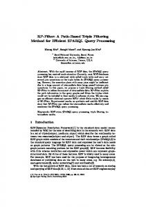
FIG. 1. The roex auditory filter shape as a function of probe level ~30–60 dB SPL in 10-dB steps! with six variable coefficients @adapted from Rosen and Baker ~1994!#.
cussion is the trade-off between number of free parameters and goodness of fit, and they conclude that a roex( p,r) model with six coefficients is the most appropriate. Specifically, their fit employed one parameter for each of p u and k, and two for each of p l and r l . The auditory filter shapes produced by this fit are shown in Fig. 1 as a function of probe level. The lower side of the filter becomes considerably broader as level increases; the upper side is invariant. Column 7 of Table I shows rms error values ~dB! obtained with the gammachirp fit using probe-dependent models with various numbers of coefficients. The integers in columns 2–6 show the number of coefficients used for the gammachirp parameter in that column. Following Rosen and Baker, we used the absolute threshold value ~22.7 dB! to limit the minimum value of P s . We also investigated
masker-dependent models, but found, like Rosen and Baker, that the rms errors were always much greater than those with the probe-dependent models. Consequently, we only consider probe-dependent models in what follows. The fit without the parameter c, i.e., the gammatone fit, is shown in the last row of Table I. The rms error is about 30% greater than that of the gammachirp fits, indicating that the gammatone filter is not suitable as an asymmetric, level-dependent filter. The rms errors in column 7 are the same for gammachirp models with between 4 and 7 variable coefficients. This indicates that the coefficients converge even with relatively few coefficients. The rms errors with the gammachirp are greater than those for roex models with six, seven, and eight variable coefficients ~compare columns 7 and 8!, and smaller for models with five variable coefficients. The gammachirp model with four variable coefficients, where n is fixed to 4, produces the same rms error as the model with five variable coefficients, where the estimated value of n is 3.89. Accordingly, the model with four variable coefficients seems sufficient to explain the masking data. Rosen and Baker do not report results with a four-coefficient model. The fixed-n model also has advantages when fitting smaller data sets and when comparing coefficients obtained with different data sets. The coefficients for the four-coefficient model are listed in row ‘‘LM 2000’’ in Table II. The auditory filter shapes produced by this fit are shown in Fig. 2 as a function of probe level. In the fitting process, the peak frequency of the amplitude spectrum varies with level, as described previously; for clarity, however, the peak frequency is normalized to 2000 Hz in the figure by adjusting the value of f r in Eq. ~2!. Below its peak frequency, the skirt of the gammachirp auditory filter broadens substantially with increasing stimulus level; above its peak frequency, the skirt sharpens a little with increasing level. These shapes are quite similar to the roex filter shapes in Fig. 1, although there are small differ-
TABLE I. Relationship between the number of filter coefficients and rms error. Columns 7 and 8 show rms ~root-mean-squared! errors in dB obtained with the gammachirp filter and the roex filter when fitting the probe-dependent model with various numbers of coefficients to all 78 data points in Rosen and Baker ~1994!. The rms errors in column 8 are calculated from the total squared errors in Rosen and Baker ~1994!. The integers in the first column show the total number of variable coefficients for both the gammachirp and the roex. The integers in other columns show the number of coefficients used for the gammachirp parameter in that column: ‘‘1’’ indicates a filter parameter that is constant across signal level and ‘‘2’’ indicates a linear dependence of the parameter on signal level. The symbol ‘‘-’’ indicates an r value of 2100 dB ~practically zero in linear terms!; ‘‘*’’ indicates an n value of 4; ‘‘—’’ indicates no model fitted at that value. The last row shows the results without parameter c, i.e., the gammatone fit.
414
Gammachirp
Number of coefficients
n
b
c
K
r
rms error
roex rms error
10 9 8
2 2 2
2 2 2
2 2 2
2 2 1
2 1 1
1.18 1.27 1.29
1.19 — 1.19
7 6 6 5 4
2 1 2 1 *
2 2 1 1 1
2 2 2 2 2
1 1 1 1 1
-
1.33 1.33 1.33 1.33 1.33
1.19 1.20 — 1.42 —
4
1
2
0
1
-
1.72
—
J. Acoust. Soc. Am., Vol. 101, No. 1, January 1997
T. Irino and R. D. Patterson: Gammachirp auditory filter
414
B. Other data sets
FIG. 2. The gammachirp auditory filter shape as a function of probe level ~30–60 dB SPL in 10-dB steps! with four variable coefficients when applied to the masking data of Rosen and Baker ~1994!. The peak frequency is normalized to 2000 Hz.
ences in the flatness around the peak frequency and in the variability of the upper skirt. Unlike the roex, the upper skirt of the gammachirp has the ‘‘backward S’’ shape observed in the dense threshold functions in Patterson ~1976!. The gammachirp filter naturally introduces the physical constraints of realistic filters into the estimation of the auditory filter shape. The derived filter shapes are also in agreement with those reported in previous studies ~Lutfi and Patterson, 1984; Patterson and Moore, 1986; Moore and Glasberg, 1987!. It also appears that we do not need the parameter r when fitting the data of LM; absolute threshold is sufficient limit to the dynamic range of the fitting process. This is another advantage of using the gammachirp fit.
Following the results in the previous subsection, we applied several probe-dependent models to the notched-noise masking data of Lutfi and Patterson ~1984! and Moore et al. ~1990!. The models with four, five, and six variable coefficients were fitted to each set of data. As before, the model with four variable coefficients proved most appropriate and so we begin with it. Given their limited size, each set of masking data was fitted with seven different sets of initial values; the set that produced coefficients giving minimum mean squared error is listed with the rms error in Table II. It is clear that the value of b converges between 1 and 2 and that c is always negatively correlated with probe level P s , as in the previous fits for LM at 2000 Hz. The filter shapes are similar to the shapes in Fig. 2 in terms of change in slope with level, except for four conditions: the filter shape is almost level independent for CP at 200 Hz and RM at 4000 Hz; the upper slope changes as much as the lower slope does for HM at 1000 and 4000 Hz. The last two rows in Table II show the means and standard deviations of the parameter values. Since the mean coefficients are close to those for LM, a ‘‘typical’’ auditory filter set resembles those shown in Fig. 2 when the peak frequencies are normalized to unity. Thus, the gammachirp with four variable coefficients provides a reasonable summary to the masking data in these data sets, although the rms errors are larger than those for the data set of LM. For completeness, we also performed the gammachirp fit with five variable coefficients ~1 n, 1 b, 2 c’s, and 1 K! and six variable coefficients ~1 b, 2 c’s, 1 K, and 2 r’s!. Only two of the models with five variable coefficients reduced the rms error more than 5%, reductions that are negligible when compared with the variance in the data sets. Since absolute threshold values were not included in these fits, the model with level-dependent r was also applied to each set ~i.e., six
TABLE II. Rms errors and coefficients obtained with the gammachirp auditory filter when fitting a probedependent model with four variable coefficients. The first column specifies the data source by the initials of the subject. CP represents data from Moore et al. ~1990!; HM, RL, RM, and WW represent data from Lutfi and Patterson ~1984!; LM represents data from Rosen and Baker ~1994!. The second column is probe frequency in Hz. The third column shows rms error in dB. The remaining columns show the best coefficients for b, c, and K with n54 and r52100 ~dB!. The last two rows show the means and standard deviations for b, c, and K.
415
Subject
Frequency
rms error
b
CP CP CP
200 400 800
4.72 2.92 2.65
1.19 1.43 1.75
20.59 2.64 2.16
HM RL RM WW
1000 1000 1000 1000
4.04 4.46 2.93 3.46
1.17 1.59 1.21 1.38
LM
2000
1.33
HM RL RM WW
4000 4000 4000 4000
mean s.d.
— —
J. Acoust. Soc. Am., Vol. 101, No. 1, January 1997
c
K 20.0097P s 20.082P s 20.070P s
2.82 21.15 24.35
8.43 4.98 5.27 3.56
20.180P s 20.146P s 20.148P s 20.098P s
23.25 211.70 27.25 26.64
1.68
3.38
20.107P s
26.08
4.14 5.10 4.94 2.75
1.85 1.75 1.50 1.79
6.31 5.17 0.61 4.18
20.153P s 20.182P s 20.019P s 20.110P s
27.67 214.39 23.63 25.87
— —
1.51 0.24
3.88 2.46
20.109P s 0.057
25.73 4.51
T. Irino and R. D. Patterson: Gammachirp auditory filter
415
variable coefficients!. All of the derived values for the parameter r were negatively correlated with probe level P s and were smaller than 240 dB, even when the signal level was 30 dB SPL. That is, the values are less than absolute threshold, and so, absolute threshold is a more suitable limit to the dynamic range when fitting these data. Moreover, the rms error was reduced more than 10% in only three cases. Thus, parameter r does not seem necessary to explain the general form of the masking data, and the model with four variable coefficients seems sufficient to explain these masking data, as well as those of Rosen and Baker. III. SUMMARY
A ‘‘gammachirp’’ function derived as an optimum auditory filter ~Irino, 1995, 1996! is shown to have an asymmetric amplitude characteristic in frequency. Using the power spectrum model of masking, and the assumption that the asymmetry is associated with stimulus level, the amplitude spectrum of the gammachirp was fitted to notched-noise masking data from 12 data sets reported in 3 different studies. A probe-dependent model with four variable coefficients is shown to provide an excellent fit to the masking data. The resultant gammachirp filter shape is similar to that obtained with a six-coefficient roex filter by Rosen and Baker ~1994!. The gammachirp has a well-defined impulse response unlike the roex auditory filter and, thus, it is an excellent candidate for an asymmetric, level-dependent auditory filterbank in time-domain models of auditory processing.3 ACKNOWLEDGMENTS
The authors wish to thank Brian C. J. Moore and Brian R. Glasberg of Cambridge University, and Stuart Rosen and Richard J. Baker of University College, London for providing their notched-noise masking data, as well as fruitful discussions. The first author wishes to thank Takesi Okadome of NTT BRL for the suggestion to study optimality of the auditory filter.
frames with a Fourier transform. There is a trade-off between the resolution of time and the resolution of frequency in this representation. The trade-off is known as the uncertainty principle, and Gabor ~1946! showed that the function which satisfies minimal uncertainty in the joint time-frequency representation is a complex sinusoidal carrier with a Gaussian envelope. This ‘‘Gabor function’’ is symmetric in time and symmetric in frequency; moreover, the frequency bands all have the same width in this time-frequency representation. The spectral analysis produced by auditory filtering differs significantly from that produced by the Fourier transform: The impulse response of the auditory filter is asymmetric in time with a fast rise and a slow decay ~de Boer and de Jongh, 1975; Carney and Yin, 1988!; the amplitude spectrum of the auditory filter is definitely not Gaussian ~Patterson, 1976!, and at high sound levels, it is asymmetric with the lower skirt shallower than the upper skirt ~Glasberg and Moore, 1990!. The gammatone function @Eq. ~1!# provides a much better fit to auditory filtering data than the Gabor function. It is clear, however, that to the extent that the gammatone differs from the Gabor function, it does not satisfy minimum uncertainty in a joint time-frequency representation of sound. Moreover, the bandwidth of the auditory filter increases with center frequency; in the region above about 500 Hz, it is essentially a ‘‘constant-Q system,’’ that is, bandwidth is proportional to center frequency ~Greenwood, 1990; Glasberg and Moore, 1990!. It is possible that the auditory system is non-optimal because it has to satisfy some mechanical or physiological constraint that is not compatible with minimal uncertainty, and which restricts the bandwidth to be a proportion of the center frequency. On the other hand, it seemed reasonable, on encountering the discrepancy between optimality and auditory filtering, to explore the possibility that the auditory system is optimal, but optimal for a different representation of sound. It is this hypothesis that led to the ‘‘scale transform’’ and the derivation of the gammachirp function. B. Scale analysis
APPENDIX A: THE DERIVATION OF THE GAMMACHIRP FUNCTION
The gammachirp function arose from consideration of the contrast between the traditional representation of sound, the spectrogram, and the representation produced by auditory filterbanks designed to mimic the spectral processing of the cochlea. The contrast is set out in Sec. A of this Appendix. It has led to the hypothesis that the time-frequency representation of sound observed at the output of the cochlea is an intervening representation produced by the auditory system to support a subsequent ‘‘scale transform,’’ and that the function that minimizes uncertainty in the time-scale representation is the gammachirp. The scale transform and the gammachirp function are the subjects of Secs. B and C, respectively. A. The spectrogram and auditory filtering
The spectrogram is a typical example of a joint timefrequency representation of sound. It is produced by converting successive segments of the sound wave into spectral 416
J. Acoust. Soc. Am., Vol. 101, No. 1, January 1997
Cohen ~1991, 1993! has suggested that ‘‘scale’’ is a physical attribute of a signal just like time and frequency, and that a time-scale representation is more appropriate than Fourier analysis for ‘‘scaled’’ signals. A ‘‘scaled’’ signal is simply one that is compressed or extended in time relative to the original, as when a tape recording is replayed at a rate faster or slower than that at which it was recorded. Cohen ~1991! introduced a ‘‘scale transform’’ in the form of an orthogonal Mellin transform ~Titchmarsh, 1948! to produce the scale representation. It is described in Sec. C. The Mellin transform converts a scaled signal into ~a! an invariant absolute distribution in the scale representation, and ~b! a value specifying the scale value of the signal. When the speed of a recording fluctuates on playback, it has a pronounced effect on the pitch we hear, but the source of the sound is not perceived to change. This suggests that the ‘‘scale’’ value and the ‘‘invariant distribution’’ of the Mellin transform may be analogous to pitch and timbre in the auditory system. Thus, the time-scale representation of sound could have distinct advantages when analyzing systems where a vibrating T. Irino and R. D. Patterson: Gammachirp auditory filter
416
source with variable rate excites a complex resonator. ‘‘Source-filter’’ models of this sort are commonly used to explain the production of sound by the vocal tract ~Fant, 1970! and musical instruments ~Fletcher and Rossing, 1991!. The scale transform can be applied to a sound wave directly. It is clear, however, that in the auditory system, the scale transform would have to be applied after auditory filtering. The wavelet transform is similar to the auditory filterbank inasmuch as it is a ‘‘constant-Q’’ system; both the envelope and the carrier of the impulse response scale with center frequency in these systems. The Mellin transform converts the individual wavelets into an invariant distribution in the scale representation. Thus, with a wavelet filterbank, when a sound is scaled, its components shift to wavelet filters that have been scaled by the same amount. So, the outputs of the scaled filters are exactly the same as the scaled versions of the outputs of the original filters. Both the scaled and unscaled filter outputs are transformed into the same distribution in the scale representation. Thus, the wavelet filterbank is ‘‘transparent’’ to the scaling of sounds, and in this sense, the wavelet transform is optimal as a preprocessor for the Mellin transform. This implies that the auditory filterbank would be a near optimum preprocessor for the Mellin transform. The optimal relationship between the Mellin transform and the wavelet transform does not uniquely determine the form of the wavelet that produces minimal uncertainty in a joint time-scale representation; Clearly, the Gabor function does not; After Cohen ~1991, 1993! adapted Klauder’s ~1980! results on affine variables in quantum mechanics to produce the scale representation for time domain functions, he showed that the optimal function for minimal uncertainty in a time-scale representation has a gamma envelope and a monotonically frequency-modulated carrier. In Cohen’s case, the instantaneous frequency of the carrier starts at infinity and converges on zero as time proceeds. This solution is not suitable for relatively narrow-band applications like auditory filtering. This led Irino ~1995, 1996! to introduce a frequency shift term that makes it possible to model the bandwidth/ center-frequency function of the auditory system, and produce a narrow-band filter centered on a specific frequency. This, in turn, led to the derivation of the gammachirp function through the optimality constraint. This, then, is the logic for the time-scale representation of sound and the gammachirp function.
C. Mathematical derivation
E
0
~A1!
s ~ t ! t p21 dt,
where p is a complex argument. One of the important properties is if s ~ t ! ⇒S ~ p ! , then s ~ at ! ⇒a 417
where j 5 A21, and exp and ln are the exponential and natural logarithmic operators. Since u a 2p S(p) u 5 u a 2 p r u • u S(p) u , the absolute distribution u S(p) u is not affected by a scaling of the signal, except for the constant that specifies the scale of the current signal; nor is it affected when the distribution is normalized. b. Minimal uncertainty and operator methods
With the Mellin transform, questions concerning minimal uncertainty in a joint representation are assessed with operator methods. They were introduced into signal processing from quantum mechanics by Gabor ~1946! because of the similarity in mathematical formalism. The following is a tutorial on operator methods based on the derivation of the Gabor function; it is adapted from Cohen ~1991, 1993!. Time and frequency operators are defined as T 5t and W 52j(d/dt) in the time domain. When the operator W is applied to the function Ae j v t , the result is
S D
W Ae j v t 5 2 j
d Ae j v t 5 v Ae j v t . dt
~A4!
Thus, for a complex exponential, the operator W introduces the frequency term v. This is the essence of operator methods. The commutator between these operators is again an operator; namely,
S DS D
@ T ,W # 5T W 2W T 5t 2 j
d d 2 2j t5 j. dt dt
~A5!
It is easy to prove by applying this operator to the function Ae j v t . Since the commutator is not zero, time and frequency do not commute. Thus, time and frequency cannot be measured independently and there is uncertainty between them, and in this case, it is Dt•D v > 21 u ^ @ T ,W # & u 5 21 u ^ j & u 5 21 ,
~A6!
where ~D.!, u.u, and ^.& denote the standard deviation, the absolute value, and the average, respectively. Functions which satisfy minimal uncertainty are solutions to the equation ~A7!
where
The Mellin transform ~Titchmarsh, 1948! of a signal, s(t) ~t.0!, is defined as S~ p !5
a 2p 5a 2 ~ p r 1 j p i ! 5a 2p r a 2 j p i 5a 2p r exp~ 2 j ln p i ! , ~A3!
~ W 2 ^ W & ! s ~ t ! 5l ~ T 2 ^ T & ! s ~ t ! ,
a. The Mellin transform
`
where the arrow ~⇒! indicates ‘‘is transformed into’’ and a is a real dilation constant. That is, the distribution S(p) is just multiplied with a constant a 2p when the function s(t) is scaled in time. If p is denoted by p r 1 j p i ,
2p
S~ p !,
J. Acoust. Soc. Am., Vol. 101, No. 1, January 1997
~A2!
l5 ^ @ T ,W # & /2~ DT ! 2 5 j/2~ Dt ! 2 .
~A8!
Using T 5t, W 52j d/dt, ^T &5^ t & , and ^W &5^v&, Eq. ~A7! is expanded as follows:
S
2j
D
j
d s ~ t ! 1lts ~ t ! 1 ~ ^ v & 2l ^ t & ! s ~ t ! 50; dt
d 2 ^ v & s ~ t ! 5l ~ t2 ^ t & ! s ~ t ! ; dt
T. Irino and R. D. Patterson: Gammachirp auditory filter
417
S
D
d 1 ^t& s~ t !1 s ~ t ! 50. 2 ts ~ t ! 1 2 j ^ v & 2 dt 2 ~ Dt ! 2 ~ Dt ! 2 ~A9! The nontrivial solution is
S
1 ^t& 2 s ~ t ! 5a exp 2 t1 j ^ v & t 2 t 1 4 ~ Dt ! 2 ~ Dt ! 2
H
5a 8 exp 2
J
S D
~A10!
c. The Mellin operator
Cohen ~1991, 1993! introduced the concept of a scale operator into signal processing in the form: C 5 21 ~ T W 1W T ! 5T W 2 21 j.
~A11!
Previously it had been known as the operator representing an affine variable in quantum mechanics ~Klauder, 1980!. The corresponding transform, that is, ‘‘the scale transform’’ ~Cohen, 1993!, is D~ c !5
A2 p
E
0
f ~ t !t
2 jc21/2
dt.
~A12!
The correspondence between the scale transform and the Mellin transform is revealed by setting p52 jc1 21 in Eq. ~A1!. Thus, Cohen’s scale transform is the Mellin transform with a specific argument. In Eq. ~A12!, the argument is restricted in range; we can, however, extend it to cover the entire complex plane by the introduction of two real constants c 0 and m as follows: p52 j ~ c2c 0 ! 1 ~ m 1 21 ! .
~A13!
s ~ t ! 5at a 2 1 jc 1 exp~ 2 a 1 t1 j v 0 t ! 5at a 2 exp~ 2 a 1 t ! exp~ j v 0 t1 jc 1 ln t ! ,
C a 5T ~ W 2 v 0 ! 1 $ c 0 1 j ~ m 2 21 ! % .
~A15!
The frequency-shift term can be removed later following consideration of the fluctuation of components at the output of the auditory filter ~Irino, 1996!. The commutator between time and this operator is @ T ,C a # 5 @ T ,C m # 5 @ T ,C # 5 jT .
APPENDIX B: THE AMPLITUDE SPECTRUM OF THE GAMMACHIRP FUNCTION
The Fourier spectrum of the gammachirp function can be derived analytically. For convenience, we consider a simplified version of the complex form of the gammachirp filter in Eq. ~2!. g c ~ t ! 5at n21 exp~ 2b 8 t ! exp~ j v r t1 jc ln t ! 5at n211 jc exp~ 2b 8 t1 j v r t !
~ C a 2 ^ C a & ! s ~ t ! 5l ~ T 2 ^ t & ! s ~ t ! , 418
J. Acoust. Soc. Am., Vol. 101, No. 1, January 1997
~A17!
~ t.0 !
~ t.0 ! ,
~B1!
where b 8 52 p b ERB( f r ), v r 52 p f r , and the phase term f is ignored. The Laplace transform of Eq. ~B1! is G C ~ s ! 5a
G ~ n1 jc ! $ s2 ~ 2b 8 1 j v r ! % n1 jc
5a
G ~ n1 jc ! u s2 ~ 2b 8 1 j v r ! u n1 jc e j u • ~ n1 jc !
5a
G ~ n1 jc ! , u s2 ~ 2b 8 1 j v r ! u e • u s2 ~ 2b 8 1 j v r ! u jc e jn u ~B2! n 2c u
where u5arg$ s2(2b 8 1 j v r ) % . Thus, the absolute value is u G C~ s !u 5
u aG ~ n1 jc ! u . u s2 ~ 2b 8 1 j v r ! u n e 2c u
~B3!
Substituting s5 j v 5 j2 p f into Eq. ~B3! to derive the amplitude of the Fourier spectrum of the gammachirp function,
~A16!
The operators in Eqs. ~A14! and ~A15! are not Hermitian except when m50; nevertheless, (C a2^C a&! is Hermitian and, thus, the eigenvalue is real. The function that satisfies minimal uncertainty between time and the quantity represented by the operator in Eq. ~A14! is the solution to the equation
~A20!
where a is a constant. The envelope t a 2 exp(2a 1 t)is a gamma distribution function g(t). The instantaneous frequency is v01c 1 /t; that is, a fractional function of time. When played as a sound, the carrier would be a chirp, and hence the name ‘‘gammachirp’’ function. When c 150, Eq. ~A20! becomes a gammatone function. Thus, the gammatone function is a first order approximation to the gammachirp function.
~A14!
Since we are concerned with signal processing by an auditory filterbank, we introduce a ‘‘frequency-shift’’ term v0 into the operator to specify the individual filters. The form of the operator becomes
d s ~ t ! 2 ~ v 0 1 j a 1 ! ts ~ t ! 1 ~ 2c 1 1 j a 2 ! s ~ t ! 50, dt ~A19!
where a15^ t & /2(Dt) 2, a25m2 212Im^ c a & 1 ^ t & 2 /2(Dt) 2 , and c 15Re^ c a & 2c 0 , Re and Im indicate the real and imaginary parts. The solution is
The corresponding Mellin operator is C m 5T W 1 $ c 0 1 j ~ m 2 21 ! % .
~A18!
Equation ~A15! expands to
D
1 ~ t2 ^ t & ! 2 exp~ j ^ v & t ! , 4 ~ Dt ! 2
`
l5 ^ @ T ,C a # /2~ DT ! 2 & 5 j ^ t & /2~ Dt ! 2 .
t 2j
where a and a 8 are constants. This is the ‘‘Gabor function,’’ and the example shows how it was derived using the constraint that the required function satisfy minimal uncertainty in a joint time-frequency representation.
1
where
u G C~ f !u 5
u aG ~ n1 jc ! u •e c u , u b 8 1 j2 p ~ f 2 f r ! u n
~B4!
where u5arg$ b 8 1 j2 p ( f 2 f r ) % . 1
Several auditory filters with gamma distribution envelopes and monotonically frequency-modulated ~FM! carriers have appeared recently. First, Lyon ~1996! has reported an ‘‘all-pole gammatone filter ~APGF!’’ based on reduction of zeros from the Laplace transform of the gammatone filter in the s plane. In this case, the intent was to simulate basilar partition motion T. Irino and R. D. Patterson: Gammachirp auditory filter
418
‘as a function of stimulus level. Although the impulse response of the APGF is not mathematically equivalent to the gammachirp function, it is similar in having a monotonic FM carrier and a gamma distribution envelope. Second, in an attempt to produce an asymmetric gammatone filter, Baker ~1995! replaced the pure-tone carrier with a monotonic FM carrier. Again, the result is not strictly a gammachirp function, but the impulse response has an FM carrier and a gamma distribution envelope. Finally, Laine and Ha¨rma¨ ~1996! have suggested similar filters for an auditory filterbank on the Bark scale. The gammachirp function can be viewed as providing the theoretical background to the larger family of auditory filters with gamma distribution envelopes and chirp carriers. 2 In their paper Rosen and Baker ~1994! presented total-squared-error values of 103.6, 105.0, 110.9, 110.9, 111.0, 111.9, and 158.1 dB2, respectively, for these conditions. 3 To construct such a filterbank, we would need to develop a mechanism to measure the output level of each filter on a moment to moment basis to specify the appropriate value of c, and thus the filter’s asymmetry, at any given moment. A mechanism of this sort has been developed by Lyon ~1982! for a nonlinear filterbank simulating cochlear mechanisms. Thus, it would not appear to be an insurmountable problem to develop one for a gammachirp filterbank. It is, however, beyond the scope of the present paper. Baker, R. ~1995!. Personal communication. Carney, L. H., and Yin, T. C. T. ~1988!. ‘‘Temporal coding of resonances by low-frequency auditory nerve fibers: single-fiber responses and a population model,’’ J. Neurophysiol. 60, 1653–1677. Cohen, L. ~1991!. ‘‘A general approach for obtaining joint representations in signal analysis and an application to scale,’’ in Advanced SignalProcessing Algorithms, Architectures, and Implementation II, edited by T. L. Franklin, Proc. SPIE, 1566, 109–133. Cohen, L. ~1993!. ‘‘The scale representation,’’ IEEE Trans. Signal Process. 41, 3275–3292. de Boer, E., and de Jongh, H. R. ~1978!. ‘‘On cochlear encoding: Potentialities and limitations of the reverse-correlation technique,’’ J. Acoust. Soc. Am. 63, 115–135. Fant, G. ~1970!. Acoustic Theory of Speech Production ~Mouton, The Hague!. Fletcher, H. ~1940!. ‘‘Auditory patterns,’’ Rev. Mod. Phys. 12, 47–65. Fletcher, N. H., and Rossing, T. D. ~1991!. The Physics of Musical Instruments ~Springer-Verlag, New York!. Gabor, D. ~1946!. ‘‘Theory of communication,’’ J. IEE ~London! 93, 429– 457. Gigue`re, C., and Woodland, P. C. ~1994!. ‘‘A computational model of the auditory periphery for speech and hearing research. I. Ascending path,’’ J. Acoust. Soc. Am. 95, 331–342. Glasberg, B. R., and Moore, B. C. J. ~1990!. ‘‘Derivation of auditory filter shapes from notched-noise data,’’ Hear. Res. 47, 103–138. Greenwood, D. D. ~1990!. ‘‘A cochlear frequency-position function for several species—29 years later,’’ J. Acoust. Soc. Am. 87, 2592–2605.
419
J. Acoust. Soc. Am., Vol. 101, No. 1, January 1997
Irino, T. ~1995!. ‘‘An optimal auditory filter,’’ in Proc. IEEE Signal Processing Society, 1995 Workshop on Applications of Signal Processing to Audio and Acoustics, New Paltz, NY. Irino, T. ~1996!. ‘‘A ‘gammachirp’ function as an optimal auditory filter with the Mellin transform,’’ in Proc. IEEE Int. Conf. Acoust., Speech Signal Processing ~ICASSP-96!, 2, 981–984, Atlanta, GA. Johannesma, P. I. M. ~1972!. ‘‘The pre-response stimulus ensemble of neurons in the cochlear nucleus,’’ in Symposium on Hearing Theory ~IPO, Eindhoven, Holland!, pp. 58–69. Klauder, J. R. ~1980!. ‘‘Path integrals for affine variables,’’ in Functional Integration: Theory and Applications, edited by J. P. Antoine and E. Tirapgui ~Plenum, New York!. Laine, U. K., and Ha¨rma¨, A. ~1996!. ‘‘On the design of Bark-FAMlet Filterbanks,’’ in Proc. Nordic Acoustical Meeting, Helsinki, Finland. Lutfi, R. A., and Patterson, R. D. ~1984!. ‘‘On the growth of masking asymmetry with stimulus intensity,’’ J. Acoust. Soc. Am. 76, 739–745. Lyon, R. F. ~1982!. ‘‘A computational model of filtering, detection, and compression in the cochlea,’’ in Proc. IEEE Int. Conf. Acoust., Speech Signal Processing ~ICASSP-82!, 1282–1285, Paris, France. Lyon, R. F. ~1996!. ‘‘The all-pole gammatone filter and auditory models,’’ in Proc. Forum Acusticum ’96, Antwerp, Belgium. Moore, B. C. J., and Glasberg, B. R. ~1987!. ‘‘Formulae describing frequency selectivity as a function of frequency and level, and their use in calculating excitation patterns,’’ Hear. Res. 28, 209–225. Moore, B. C. J., Peters, R. W., and Glasberg, B. R. ~1990!. ‘‘Auditory filter shapes at low center frequencies,’’ J. Acoust. Soc. Am. 88, 132–140. Patterson, R. D. ~1976!. ‘‘Auditory filter shapes derived with noise stimuli,’’ J. Acoust. Soc. Am. 59, 640–654. Patterson, R. D. ~1994!. ‘‘The sound of a sinusoid: Spectral models,’’ J. Acoust. Soc. Am. 96, 1409–1418. Patterson, R. D., Allerhand, M., and Gigue`re, C. ~1995!. ‘‘Time-domain modelling of peripheral auditory processing: a modular architecture and a software platform,’’ J. Acoust. Soc. Am. 98, 1890–1894. Patterson, R. D., and Moore, B. C. J. ~1986!. ‘‘Auditory filters and excitation patterns as representations of frequency resolution,’’ in Frequency Selectivity in Hearing, edited by B. C. J. Moore ~Academic, London!. Patterson, R. D., and Nimmo-Smith, I. ~1980!. ‘‘Off-frequency listening and auditory filter asymmetry,’’ J. Acoust. Soc. Am. 67, 229–245. Patterson, R. D., Nimmo-Smith, I., Weber, D. L., and Milroy, R. ~1982!. ‘‘The deterioration of hearing with age: Frequency selectivity, the critical ratio, the audiogram, and speech threshold,’’ J. Acoust. Soc. Am. 72, 1788–1803. Press, W. H., Flannery, B. P., Teukolsky, S. A., and Vetterling, W. T. ~1988!. Numerical Recipes in C ~Cambridge U.P., Cambridge!. Rosen, S., and Baker, R. J. ~1994!. ‘‘Characterising auditory filter nonlinearity,’’ Hear. Res. 73, 231–243. Titchmarsh, E. C. ~1948!. Introduction to the Theory of Fourier Integrals ~Oxford U.P., London!, 2nd ed.
T. Irino and R. D. Patterson: Gammachirp auditory filter
419