mon to many fields in engineering and physics like electromagnetism, acoustics, and optics. Many differ ... essential relations with only a basic knowledge in sig-.
A TUTORIAL ON THE REPRESENTATION OF TWO-DIMENSIONAL WAVE FIELDS BY MULTIDIMENSIONAL SIGNALS Rudolf Rabenstein, Peter Steffen, Sascha Spors University Erlangen-Nuremberg, Multimedia Communications and Signal Processing, Cauerstr. 7, D-91058 Erlangen, Germany {rabe, steffen, spors }@LNT.de
ABSTRACT The representation of information by waves is common to many fields in engineering and physics like electromagnetism, acoustics, and optics. Many different tools for the description of wave-like signals have been developed. Most of them are based on methods and results from mathematical physics with different viewpoints according to the specific application areas. This tutorial presents a framework for some of the most common of these representations. It is based on well-known transform domain signal descriptions from multidimensional systems theory. 1. INTRODUCTION Waves play a dominant role in the transmission of information over time and space. Their propagation is governed by the wave equation. It is the foundation of many applications in acoustics, optics, and electromagnetism. Solutions of the wave equation are called wave fields. This tutorial derives various representations of wave fields. The purpose is to provide a framework for the essential relations with only a basic knowledge in signals and systems. The components of this framwork are the wave equation and Fourier transforms, Fourier series, and Dirac impulses in one and two dimensions. This contribution is an abridged version of [1]. The representations in this tutorial are embedded in a time-dependent, spatially three-dimensional description. However, only an important special case is considered here, namely that the spatial signals are separable in one of the three spatial coordinates. This assumption allows a reduction to two-dimensional wave fields which is important for all applications where the transmitters and receivers are located in a plane. Therefore, only the two-dimensional case is presented here. Sections 2 and 3 review some well-known facts
about one-dimensional signals and systems and introduce the same notions for multidimensional signals and systems, respectively. Sec. 4 specifies these results for wave fields, i.e. for signals which satisfy the wave equation. The so-called plane wave solution is considered in detail and it is shown how to represent also the general solution of the wave equation by plane waves. The resulting representations are derived for different coordinate systems. Finally the results are compiled to highlight the developed framework for the representation of two-dimensional wave fields. 2. ONE-DIMENSIONAL SIGNALS This section reviews some well-known one-dimensional signal transforms with respect to time, space, angular, and radial coordinates. These remarks serve as reference for the multidimensional case in Sec. 3. 2.1. Fourier Transform For the time variable t and the temporal frequency variable ω, the Fourier transform is given by F{f (t)} = F (ω) =
Z∞
f (t)e−jωt dt ,
(1)
Z∞
(2)
−∞
F
−1
1 {F (ω)} = f (t) = 2π
F (ω)ejωt dω .
−∞
The Fourier transform applies also to functions of the space variable x and the spatial frequency variable kx T{f (x)} = f˜(kx ) =
Z∞
f (x)e−jkx x dx ,
(3)
−∞
T
−1
1 {f˜(kx )} = f (x) = 2π
Z∞
−∞
f˜(kx )ejkx x dkx . (4)
2.2. Fourier Series
1 Sϕ {f (ϕ)} = f˚(ν) = 2π
f (ϕ)e−jνϕ dϕ ,
(5)
f˚(ν)ejνϕ .
(6)
ν
g
Periodic functions f (ϕ) of the angle ϕ with period 2π can be expressed by the complex expansion coefficients f˚(ν) as Z2π
P
=
f (ϕ)
f˚(ν) ejνϕ 7
Sϕ Figure 2: Representation of the Fourier series expansion Sϕ ((5,6)
0
˚ S−1 ϕ {f (ν)} = f (ϕ) =
∞ X
ν=−∞
Of special importance in this context are the following Fourier series expansions leading to Bessel functions Sα {e+jkr cos(θ−α) } = j ν e−jνθ Jν (kr) , Sθ {e
−jkr cos(θ−α)
} = j
e
−ν −jνα
(7)
sional (MD) signals, specifically to signals which depend on time and two spatial coordinates. For the spatial coordinates, two different coordinate systems are considered, namely Cartesian and polar coordinates. Signals in polar coordinates may be expanded into a Fourier series with respect to the polar angle (angular expansion).
Jν (kr) . (8)
2.3. Fourier-Bessel (Hankel) Transform
3.1. Time and space dependent signals
The ν-th order Fourier-Bessel transform (Hankel transform) of a function f (r) for r > 0 is given by [2, 3]
The Cartesian and polar coordinates are written as
Hν {f (r)} = fˆν (k) =
Z∞
f (r)Jν (kr) r dr ,
Hν−1 {fˆν (k)} = f (r) =
Z∞
fˆν (k)Jν (kr) k dk . (10)
x= (9)
0
Figs. 1 and 2 compile graphical representations of the Fourier transforms with respect to time (1,2) and space (3,4), of the Fourier-Bessel transform (9,10), and of the Fourier series expansion (5,6). These relations will appear as building blocks of the corresponding multidimensional representations in Sec. 3. f (t) O
F �
F (ω)
f (x) O �
T
f˜(kx )
x y
�
,
r=
�
r α
�
(11)
respectively. The relations between Cartesian and polar coordinates are given by
0
2.4. Representations of one-dimensional signals
�
x=r
�
cos α sin α
�
,
r=
" p
x2 +� y 2� y arctan x
#
. (12)
Functions of time and of space in Cartesian coordinates are denoted by the subscript c as fc (t, x). Similarly functions of time and of space in polar coordinates are written as fp (t, r). The same spatial shape can be equally described in Cartesian and in polar coordinates, i.e. fc (t, x) = fp (t, r) .
f (r) O
�
Hν
fˆν (k)
Figure 1: Representations of the Fourier transform F and T with respect to time and space domain (1–4) and of the Fourier-Bessel (Hankel) transform Hν (9,10)
3.2. Fourier Transform with respect to time The Fourier transforms of fc (t, x) and fp (t, r) with respect to time are denoted by Fc (ω, x) = F{fc (t, x)} and Fp (ω, r) = F{fp (t, r)}.
3.3. Fourier Transform with respect to space 3. MULTIDIMENSIONAL SIGNALS The transforms for one-dimensional signals introduced in the previous section are now applied to multidimen-
The Fourier transform with respect to space takes different forms for Cartesian and polar coordinates. They are denoted by Tc and Tp , respectively. The Fourier transform Tc {fc (t, x)} with respect to
space is defined by Z∞ Z∞
f˜c (t, k) =
fc (t, x)e−j(x,k) dx dy ,
−∞ −∞ Z∞
1 fc (t, x) = 2 4π
Z∞
(13)
f˜c (t, k)ej(x,k) dkx dky . (14)
−∞ −∞
k = [kx , ky ]T is the vector of spatial angular frequencies (wave numbers) and (x, k) is the scalar product (x, k) = kT x = kx x + ky y .
(15)
The Fourier transform pair for polar coordinates is obtained from the Cartesian version in (13,14) by substitution of the Cartesian variables x by the polar variables r according to (12). With a polar version p of the vector k � � ky k , (16) p= , k = |k|, tan θ = θ kx the spatial Fourier transform Tp {fp (t, r)} in polar coordinates becomes f˜p (t, p) =
Z2π Z∞ 0
fp (t, r)e−j r dr dα
(17)
0
1 fp (t, r) = 2 4π
Z2π Z∞ 0
f˜p (t, p)ej k dk dθ. (18)
0
When x0 and r0 are related as in (11, 12) then δc (x − x0 ) = δp (r − r0 ). Dirac impulses in the frequency domain for Cartesian and polar coordinates are defined by δc (k − k0 ) = δ(kx − k0,x )δ(ky − k0,y ) , 1 δp (p − p0 ) = δ(k − k0 )δ(θ − θ0 ) . k0
(23)
3.5. Multidimensional Fourier Transform Application of the Fourier transforms with respect to time and space defines a multidimensional Fourier transform denoted by FT F˜c (ω, k) = FT c {fc (t, x)} =Tc {F{fc (t, x)}} (24) F˜p (ω, p) = FT p {fp (t, r)} =Tp {F{fp (t, r)}} (25) 3.6. Angular Expansions The functions Fp (ω, r) and F˜p (ω, p) are periodic in α and in θ, respectively. Therefore, they can be expanded into Fourier series with respect to α and θ using the properties (7,8) ˚p (ω, r, ν) = Sα {Fp (ω, r)} , F ˚ ˜ p (ω, k, ν) = Sθ {F˜p (ω, p)} . F
(26) (27)
˚ ˜ p (ω, k, ν) can be expressed as Then F
The scalar product (15) becomes in polar coordinates
˚ ˜ p (ω, k, ν) = Sθ {Tp {Fp (ω, r)}} = F
(x, k) = kr cos(θ − α) =< r, p > .
Z∞ Z2π
(19) =
3.4. Two-Dimensional Dirac Impulses
(22)
(28)
Fp (ω, r) Sθ {e−j } dα r dr .
0
0
defines for f˜c (t, k) ≡ With (8) and (26) follows a relation between the angu1 the two-dimensional Dirac impulse [4] in Cartesian ˚ ˚p (ω, r, ν) and F ˜ p (ω, k, ν) lar expansions F coordinates δc (x − x0 )
The inverse Fourier transform Tc−1
δc (x − x0 ) = δ(x − x0 )δ(y − y0 ) = Z∞ Z∞ 1 = 2 ej(x−x0 ,k) dkx dky . (20) 4π −∞ −∞
δ(x) denotes the one-dimensional Dirac impulse. By substitution of the Cartesian with polar coordinates follows the two-dimensional Dirac impulse in polar coordinates δp (r − r0 ) =
1 δ(r − r0 )δ(α − α0 ) . r0
(21)
˚ ˜ p (ω, k, ν) = F
Z∞
˚p (ω, r, ν) 2π Jν (kr) r dr . (29) F jν
0
Since this relation bears close resemblance with the Hankel transform (9), it is called a modified Hankel transform Hν . An approach analogous to (28) for ˚p (ω, r, ν) = Sα {T −1 {F˜p (ω, p)}} F p leads to a relation inverse to (29). Thus the modified ˚ ˚p (ω, r, ν)} = F ˜ p (ω, k, ν) is Hankel transform Hν {F
given by
4. WAVE FIELDS
˚ ˜ p (ω, k, ν) = F
Z∞
˚p (ω, r, ν) 2π Jν (kr) r dr , (30) F jν
˚p (ω, r, ν) = F
Z∞
˚ ˜ p (ω, k, ν) j Jν (kr) k dk . (31) F 2π
0
ν
0
3.7. Representations of Multidimensional Signals The sections above have developed the relations between MD signals in Cartesian and polar coordinates and in various transform domains. The resulting representation of MD signals and the relations between +3 denotes them are compiled in Figs. 3 and 4 ( ks conversion between Cartesian and polar coordinates.)
After having introduced various representations of general MD signals, the results are specialized to a certain class of signals. From now on only those signals are considered which satisfy the wave equation. This restriction poses strong constraints on the admissible signals by closely relating their variations in time and space. The formulations for these constraints depend on the chosen domain and are explored in the sequel. Signals which satisfy the wave equation are also called solutions of the wave equation or wave fields or simply waves. They are denoted by pc (t, x) or by the corresponding notations according to Fig. 4. First, signals in Cartesian coordinates will be considered, then follow polar coordinates and Fourier series expansions. 4.1. The Wave Equation
x=
�
x y
O
�
+3 r = ks
�
r α
O
k=
Sα o
Hν
�
kx ky
/ (r, ν) O
Tp
Tc ��
�
�
+3 p = ks
�
k θ
�
�
Sθ o
/ (k, ν)
Figure 3: Coordinates in the space domain and in the spatial frequency domain in different coordinate systems.
fc (t, x)
=
=
fp (t, r)
O
O
ν
e
Fc (ω, x) = Fp (ω, r) = O
O
�
e
Tp
Tc
8 O
F �
� �
f˚p (t, r, ν) ejνα
Sα
F
F
P
P ν
˚p (ω, r, ν) ejνα F 8 O
Sα
Hν �
�
P ˚ F˜c (ω, k) = F˜p (ω, p) = F˜ p (ω, k, ν) ejνθ f
ν
7
The wave equation is given by ∆pc (t, x) −
1 ∂2 pc (t, x) = 0 . c2 ∂t2
(32)
∆ = ∇2 denotes the Laplace operator [5]. Application of the Fourier transform F with respect to time turns the wave equation into the Helmholtz equation ∆Pc (ω, x) +
� ω �2
Pc (ω, x) = 0 .
c
(33)
Application of the Fourier transform Tc with respect to space leads to a multiplication with (jk)T (jk) = −k 2 −k 2 P˜c (ω, k) +
� ω �2 c
P˜c (ω, k) = 0 .
(34)
In the spatial and temporal frequency domain, the constraint on the possible solutions of the wave equation consists of a strong coupling between the temporal frequency variable ω and the magnitude k of the spatial frequency variable k, i.e. P˜c (ω, k) = 0
for
k 2 6=
ω2 . c2
The following sections explain how this constraints affect the various representations from Fig. 4.
Sθ
4.2. Plane Wave Solution of the Wave Equation Figure 4: Representations of MD signals in the time and space domain and in the corresponding frequency domains in different coordinate systems
A plane wave is a special solution of the wave equation, which has a very simple form for Cartesian coordinates. It is determined by its waveform and by the direction from which the waveform emanates. The
ky
waveform is given by a time function g0 (t) and the direction is given by the unit vector n0 � � � � n0,x cos θ0 n0 = = . PSfrag (35)replacements n0,y sin θ0 The plane wave solution is the MD signal � � 1 pc,0 (t, x) = g0 t + (x, n0 ) , c
k0 = k0,y
ω c
n0 θ0
k0,x
kx
(36)
where (x, n0 ) is the scalar product between x and n0 . It describes a planar wave front which propagates through space from the direction of n0 with speed c. In the origin x = 0, the wave form g0 (t) is observed directly as Figure 5: Possible locations of the Dirac impulse pc,0 (t, 0) = g0 (t). δc (k − k0 ) in the kx –ky –plane Now the Fourier transforms F and Tc with respect ω to time and space are applied to the plane wave solution. First, Fourier transform F with respect to time gives Pc,0 (ω, x) = G0 (ω)ej c (x,n0 ) = G0 (ω)ej(x,k0 ) (37) ω
ky
where k0 is the spatial frequency vector in the direcPSfrag replacements tion n0 from where the plane wave is emitted. � � � � ω n0,x k0,x = , k 0 = n0 = k 0 n0 = k 0 n0,y k0,y c 2 2 k0,x + k0,y = k02 =
ω2 . c2
(38)
Next, spatial Fourier transform Tc gives with (22) P˜c,0 (ω, k) = 4π 2 G0 (ω)δc (k − k0 ) .
(39)
Equation (39) shows that temporal and spatial frequency variables in P˜c,0 (ω, k) are closely related. Waves have a spatial spectrum which is rather restricted, i.e. it is a 2D Dirac pulse in the kx –ky –plane. The distance from the origin is given by the temporal frequency ω due to |k0 | = ω/c. The direction is determined by the direction of wave emanation n0 . Fig. 5 shows the possible locations of δc (k − k0 ). 4.3. General Solution of the Wave Equation The wave equation admits more general solutions than the plane wave solution discussed above. However, the general solution may be obtained by superimposing plane waves from all possible directions (0 ≤ θ0 < 2π) and with varying waveforms. To express the dependency on the angle θ0 properly, the plane wave solution (39) is rewritten as P˜c,0 (ω, k) = P˜c (ω, θ0 , k) = 4π 2 G(ω, θ0 )δc (k − k0 ) . (40)
kx
Figure 6: Support of the Dirac impulse δc (k − k0 ) in the (ω, kx , ky )–domain The general solution is obtained by integration over all possibe directions θ0 P˜c (ω, k) =
Z2π
P˜c (ω, θ0 , k) dθ0 =
0
= 4π
2
Z2π
G(ω, θ0 )δc (k − k0 ) dθ0 .
(41)
0
This construction of the general solution is straightforward, but it is not compatible with either a Cartesian or a polar coordinate system. While the spatial frequency vector k is formulated in Cartesian coordinates, the angle dependence in G(ω, θ0 ) corresponds to polar coordinates. In the sequel, equation (41) is expressed first in Cartesian and then in polar coordinates. 4.3.1. Cartesian coordinates To express (41) in Cartesian coordinates, the angle θ0 has to be substituted by k0,x (or k0,y ). It is of advantage
to break the integral from 0 to 2π into two integrals ˜ (1) (ω, k0,x ) for from 0 to π and π to 2π. Introducing G ˜ (2) (ω, k0,x ) for π ≤ θ0 < 2π 0 ≤ θ0 < π and G � G(ω, θ0 ) |k0,x | ≤ k0 (1) ˜ G (ω, k0,x ) = , (42) 0 |k0,x | > k0 � ˜ (2) (ω, k0,x ) = −G(ω, θ0 ) |k0,x | ≤ k0 , (43) G 0 |k0,x | > k0 and following the standard procedures for the substitution in integrals leads to P˜c (ω, k) = P˜c(1) (ω, k) + P˜c(2) (ω, k) ,
(44)
with (for i = 1, 2)
(49)
This representation shows, that the spatially 2D spectrum P˜c (ω, k) exists only on the region of support in the (ω, kx , ky )–domain indicated in Fig. 6. The inverse transformation Tc−1 with respect to k gives 1 Pc (ω, x) = 2π
Z∞
˜ c (ω, kx )e H
� � q 2 j kx x+ ( ωc ) −kx2 y
dkx .
−∞
P˜c(i) (ω, k) = Z∞ 2 ˜ (i) (ω, k0,x ) q 1 δc (k − k0 ) dk0,x . 4π G 2 − k2 k 0 0,x −∞
(45)
The two terms in (44) have a physical interpretation as waves emanating from opposite directions. Since both terms have an identical structure, they will not be further distinguished from now on. The results derived below apply to either term with proper definition of ˜ G(ω, k0,x ) according to (42) or (43). Equation (45) shows that the 2D spatial Fourier transform P˜c (ω, k) is generated by a signal with one spatial dimension only. Denoting the Fourier transform of this signal by ˜ c (ω, k0,x ) = G(ω, ˜ H k0,x ) q
2π � ω 2 2 − k0,x c
(46)
gives equation (45) the concise form (the superscript (i) now omitted) P˜c (ω, k) = 2π
Performing the 1D integration in (47) yields ! r� � 2 ω ˜ c (ω, kx ) δ ky − P˜c (ω, k) = 2π H − kx2 . c
Z∞
˜ c (ω, k0,x )δc (k − k0 ) dk0,x . H
−∞
(47)
(50) Equation (50) establishes the connection between a general solution of the wave equation Pc (ω, x) and the 1D ˜ c (ω, kx ). This relation can spatial Fourier spectrum H be understood more clearly, if P˜c (ω, x) is restricted to its values on the x-axis, i.e. y = 0. Then (50) turns into a one-dimensional inverse Fourier transform with respect to space according to (4) ˜ c (ω, kx )} , (51) Pc (ω, x)|y=0 = Hc (ω, x) = T −1 {H The relations shown above give rise to the following interpretations: From (51) follows ˜ c (ω, kx ) = T{Hc (ω, x)} = T{ Pc (ω, x)| }. H y=0 (52) This relation along with (50) shows that a spatially 2D wave field is completely determined by its values along a line in the x-y plane, i.e. a spatially 1D signal. For the derivation given here, this line is the x-axis, but by suitable coordinate transformations the representation could be extended to other lines in the x-y plane which are not orthogonal to n0 . From (46) follows r� � 1 ω 2 ˜ ˜ c (ω, kx ) G(ω, kx ) = H − kx2 , (53) 2π c
To show the relation between P˜c (ω, k) and its spaThe values along the x-axis are related by (53) to the ˜ c (ω, k0,x ), the definition of the tially 1D counterpart H Fourier spectrum of the waveform of plane waves from Dirac impulse (22) and the dispersion relation accorddifferent angles of incidence. This relation can be ining to (38) are used ˜ terpreted as a projection of the waveform spectra G(ω, kx ) ! r� � to the kx -axis of the Cartesian coordinate system. ω 2 2 Equation (49) shows that the frequency domain repδc (k − k0 ) = δ(kx − k0,x ) δ ky − − k0,x . c resentation P˜ (ω, k) of a wave field is nonzero only on a cone in the (ω, kx , ky )–domain as shown in Fig. 6. (48)
The relations developed in this subsection are the specialization of the the 2D Fourier transform Tc for general MD signals to solutions of the wave equation. They are also known as plane wave expansion or plane wave decomposition (see e.g. [6]). 4.3.2. Polar coordinates To formulate these results in polar coordinates, the general solution of the wave equation in the form of (41) is reconsidered. Converting it from Cartesian to polar coordinates results in [1] P˜p (ω, p) = 4π 2
Z2π
G(ω, θ0 )δp (p − p0 ) dθ0 . (54)
0
Observing (23) and carrying out the integration in (54) yields ω� 1 � . P˜p (ω, p) = 4π 2 G(ω, θ) δ k − k c
(55)
As in the Cartesian case the frequency domain representation P˜p (ω, p) is nonzero only on a cone in the (ω, kx , ky )–domain or in the (ω, k, θ)–domain respectively (see Fig. 6). This condition is mathematically represented by the Dirac impulse incorporating the dispersion relation in (55). By inverse Fourier transformation Pp (ω, r) = Tp−1 {P˜p (ω, p)} with respect to space follows Pp (ω, r) =
Z2π
G(ω, θ)ej c r cos(θ−α) dθ . ω
(56)
0
As for Cartesian coordinates in (50), the wave field in polar coordinates is generated by a spatially 1D signal. Here, this signal is given by the waveform spectrum G(ω, θ). 4.3.3. Angular Expansions ˚p (ω, r, ν) of Pp (ω, r) and The Fourier coeffients P ˚ ˜ p (ω, k, ν) of P˜p (ω, p) follow from a Fourier series P expansion of the wave field description in polar coordinates according to (54) and (56). The coefficients ˚p (ω, r, ν) = Sα {Pp (ω, r)} are given by P ˚p (ω, r, ν) = P
Z2π
G(ω, θ0 ) Sα {ej c r cos(θ0 −α) } dθ0 . ω
0
(57)
With (7) follows � � ˚ ν) ˚p (ω, r, ν) = 2πj ν Jν ω r G(ω, P c
(58)
with the Fourier coefficients of G(ω, θ) ˚ ν) = Sθ {G(ω, θ)} = 1 G(ω, 2π
Z2π
G(ω, θ)e−jνθ dθ .
0
(59) ˚p (ω, r, ν) of the spatially 2D The Fourier coefficients P signal Pp (ω, r) can be represented in terms of the Fourier ˚ ν) of the spatially 1D signal G(ω, θ). coefficients G(ω, There are two ways to calculate the coefficients ˚ ˜ P p (ω, k, ν) of P˜p (ω, p) (see Fig. 4). One way is to apply Sθ directly to P˜p (ω, p). The second way is to apply the modified Hankel transform Hν to the Fourier ˚p (ω, r, ν). In either case, the result is [1] coefficients P � � ˚ ˜ p (ω, k, ν) = 4π 2 G(ω, ˚ ν) 1 δ k − ω . P k c
(60)
˚ ˜ p (ω, k, ν) of the spaAgain, the Fourier coefficients P ˜ tially 2D signal Pp (ω, p) can be represented in terms ˚ ν). of the Fourier coefficients G(ω, 4.4. Compilation of the Results The properties of MD signals which describe wave fields are now compiled in concise form. The contents of table 1 specify the properties of the general signals from Fig. 4 for the case that they satisfy the wave equation. The spatially two-dimensional signals which solve the wave equation can be represented by a spatially onedimensional quantity. This statement holds for all considered coordinate systems and for both space and spatial frequency domains. This one-dimensional quantity can be derived directly from the general solution constituted by the wave forms of plane waves from all directions. These wave forms appear either directly as their temporal Fourier transform G(ω, θ), its Fourier ˚ ν), or as the projection H ˜ c (ω, kx ) of coefficients G(ω, G(ω, θ) to the kx –axis of the coordinate system of the spatial frequency domain. This projection corresponds to the values Hc (ω, x) of the wave field Pc (ω, x) along the x–axis. 5. CONCLUSIONS A framework for the representation of two-dimensional signals in different coordinate systems and different
Cartesian Coordinates 1 Pc (ω, x) = 2π
Z∞
˜ c (ω, kx )e H
� � q 2 j kx x+ ( ωc ) −kx2 y
dkx
−∞
Pc (ω, x)|y=0 = Hc (ω, x)
� q ˜ Pc (ω, k) = 2π δ ky − 1 ˜ ˜ G(ω, kx ) = Hc (ω, kx ) 2π
Polar Coordinates Pp (ω, r) =
Z2π
G(ω, θ)ej c r cos(θ−α) dθ ω
0
Fourier Series Coefficients � � ˚p (ω, r, ν) = 2πj ν Jν ω r G(ω, ˚ ν) P c
� ω 2 c q
−
� ω 2 c
kx2
�
˜ c (ω, kx ) H
− kx2
1 � ω� P˜p (ω, p) = 4π 2 G(ω, θ) δ k − k c
� � ˚ ˜ p (ω, k, ν) = 4π 2 G(ω, ˚ ν) 1 δ k − ω P k c
Table 1: Representation of a wave field in the space domain (left) and in the spatial frequency domain (right) transform domains has been developed. It comprises known results for wave fields as usually derived in the fields of imaging and acoustics. By adopting a general viewpoint from the theory of signals and systems, these results could be derived in a straightforward fashion and without resorting to special applications. 6. REFERENCES [1] R. Rabenstein, P. Steffen, and S. Spors, “Representation of two-dimensional wave fields by multidimensional signals,” Signal Processing, to be published. [2] A. Papoulis, Systems and Transforms with Applications in Optics, McGraw-Hill, 1968. [3] I.N. Sneddon, The Use of Integral Transforms, McGraw-Hill, New York, 1972. [4] J.D. Gaskill, Linear Systems, Fourier Transforms, and Optics, John Wiley & Sons, 1978. [5] I.S. Gradshteyn and I.M. Ryzhik, Tables of Integrals, Series, and Products, Academic Press, 2000. [6] E.G. Williams, Fourier Acoustics: Sound Radiation and Nearfield Acoustical Holography, Academic Press, 1999. [7] A.J. Berkhout, Applied Seismic Wave Theory, Elsevier, 1987. [8] David T. Blackstock, Fundamentals of Physical Acoustics, J. Wiley & Sons, 2000.
[9] R.N. Bracewell, Kluwer, 2003.
Fourier Analysis and Imaging,
[10] D. E. Dudgeon and R. M. Mersereau, Multidimensional Digital Signal Processing, Prentice-Hall, Englewood Cliffs, USA, 1984. [11] D.H. Johnson and D.E. Dudgeon, Array Signal Processing: Concepts and Techniques., Prentice-Hall, 1993. [12] J.A. Scales, Theory of Acoustic Imaging, Samizdat Press, 1997. [13] M. Brandstein and D. Ward, Eds., Microphone Arrays, Springer, 2001. [14] Y. Huang and J. Benesty, Eds., Audio Signal Processing for Next-Generation Multimedia Communication Systems, Kluwer Academic Press, Boston, USA, 2004. [15] J. Coleman, “Ping-pong sample times on a linear array halve the Nyquist rate,” in Proc. Int. Conf. on Speech, Acoustics, and Signal Processing (ICASSP). IEEE, 2004. [16] A.J. Berkhout, “A holographic approach to acoustic control,” Journal of the Audio Engineering Society, vol. 36, pp. 977–995, December 1988. [17] A.J. Berkhout, D. de Vries, and P. Vogel, “Acoustic control by wave field synthesis,” Journal of the Acoustic Society of America, vol. 93, no. 5, pp. 2764–2778, May 1993.