A Uniform Approach for Modeling. Electrical Machines. Michael Beuschel.
Abstract. In this paper, an approach is presented that enables uniform modeling
of ...
0��%HXVFKHO� $�8QLIRUP�$SSURDFK�IRU�0RGHOLQJ�(OHFWULFDO 0DFKLQHV� 0RGHOLFD�:RUNVKRS������3URFHHGLQJV��SS����������
3DSHU�SUHVHQWHG�DW�WKH�0RGHOLFD�:RUNVKRS�������2FW�����������������/XQG��6ZHGHQ� $OO�SDSHUV�RI�WKLV�ZRUNVKRS�FDQ�EH�GRZQORDGHG�IURP KWWS���ZZZ�0RGHOLFD�RUJ�PRGHOLFD�����SURFHHGLQJV�KWPO :RUNVKRS�3URJUDP�&RPPLWWHH� � 3HWHU�)ULW]VRQ��3(/$%��'HSDUWPHQW�RI�&RPSXWHU�DQG�,QIRUPDWLRQ�6FLHQFH��/LQN|SLQJ 8QLYHUVLW\��6ZHGHQ��FKDLUPDQ�RI�WKH�SURJUDP�FRPPLWWHH � � 0DUWLQ�2WWHU��*HUPDQ�$HURVSDFH�&HQWHU��,QVWLWXWH�RI�5RERWLFV�DQG�0HFKDWURQLFV� 2EHUSIDIIHQKRIHQ��*HUPDQ\� � +LOGLQJ�(OPTYLVW��'\QDVLP�$%��/XQG��6ZHGHQ� � +XEHUWXV�7XPPHVFKHLW��'HSDUWPHQW�RI�$XWRPDWLF�&RQWURO��/XQG�8QLYHUVLW\��6ZHGHQ� :RUNVKRS�2UJDQL]LQJ�&RPPLWWHH� � +XEHUWXV�7XPPHVFKHLW��'HSDUWPHQW�RI�$XWRPDWLF�&RQWURO��/XQG�8QLYHUVLW\��6ZHGHQ� � 9DGLP�(QJHOVRQ��'HSDUWPHQW�RI�&RPSXWHU�DQG�,QIRUPDWLRQ�6FLHQFH��/LQN|SLQJ 8QLYHUVLW\��6ZHGHQ�
A Uniform Approach for Modeling Electrical Machines Michael Beuschel
Abstract In this paper, an approach is presented that enables uniform modeling of different types of electrical machines using a novel Modelica library of magnetic components. Results of simulations with Dymola are presented. This approach is also applicable to education.
magnetic potential difference ∆θx , ∆θy are used in 2-dimensional space vector representation including real and imaginary part (x- and y-axis respectively). This is reflected by the definition of magnetic connectors MagP and MagN, which only have different icons to identify more easily the pins of a component (see Fig. 1).
2.2 Basic Magnetic Components
1
Introduction
Modelica provides a very general approach of modeling physical systems. Libraries for electrical and electronic as well as for mechanical components are already distributed on an open source code basis. Based on this, a new library1 for modeling rotational magnetic fields has been developed also including interfaces to electrical and mechanical components. In this paper, rotary electro-magnetic motors are considered. Basically, different types of electrical machines employ the same physical principle: A magnetic field is produced that always tends towards a state of minimal energy. This is achieved by a change of the rotor position, which is the desired effect of a motor.
2
A Modelica Library of Magnetic Components
Calculation of magnetic circuits is often done using a notation similar to that of electrical circuits. Therefore, the magnetic flux ψ and the magnetic potential difference ∆θ can be treated like current i and voltage v respectively. These are used in the following to model magnetic components.
2.1
Magnetic Connectors
As the focus of this paper is on modeling rotating electrical machines, both magnetic flux ψx , ψy and 1 For
details on the Modelica implementation, please see the appendix.
Some basic magnetic components have been implemented (see Fig. 1).
�
�
�
As in electrical circuits, a magnetic ground (MagGround) is mandatory in every magnetic circuit model to define the “magnetic potential” for simulation.2 θx
=
0
θy
=
0
(1)
A permanent magnet is a magnetic source (MagSource), that generates a magnetic potential difference ∆θ with angular orientation β. ∆θx
=
∆θ cos(β)
∆θy
=
∆θ sin(β)
(2)
A linear magnetic resistance (MagResistance) connects the magnetic potential difference with the magnetic flux by
with
ψx Rm
=
∆θx
ψy Rm
=
∆θy
=
2
Rm
(3)
N =M
The magnetic resistance Rm is determined by the number N of turns and the corresponding (electrical) inductance M. For 2-dimensional simulation, the above operation is calculated for the real and imaginary part of the magnetic field separately.
Figure 1: Basic magnetic components
system. This is why the negative mechanical angle Zϕ is used here instead of β. Z scales the mechanical angle to obtain the magnetic one, where Z is half the number of poles. The mechanical connector flange b can be connected to components of the Modelica.Mechanics.Rotational library.
2.5 Stator and Rotor Employing basic magnetic components, interfaces to electrical and mechanical components are discussed To model the interaction between the stationary and rotational part of electrical machines, a stator rotor in the next section (see Fig. 2). block (StatorRotor) is employed. It provides transformation between stator and rotor coordinates and calculates the mechanical torque τ from magnetic flux ψx , ψy and potential difference ∆θx , ∆θy .
Figure 2: Magnetic interface components
2.3
0
=
ψ1x
+
ψ2x cos(Z ϕ)
0
=
ψ1y
+
ψ2x sin(Z ϕ) + ψ2y cos(Z ϕ) (6)
∆θ1x
=
∆θ2x cos(Z ϕ)
∆θ1y
=
∆θ2x sin(Z ϕ) + ∆θ2y cos(Z ϕ)
τ
=
Z ψ2x ∆θ2y
+
ψ2y sin(Z ϕ)
∆θ2y sin(Z ϕ) Z ψ2y ∆θ2x
(7) (8)
Magnetic Coupling
A linear magnetic coupling (MagCoupling) is based on the electrical OnePort class. It relates electrical voltage v and current i to magnetic potential difference 3 Modeling Electrical Machines Usand flux due to the induction law. An additional scaling the Magnetics Library ing factor k adjusts magnetic to electrical values due to simplified modeling and field geometry. The components of the magnetics library have been � � tested implementing common electrical machines in dψy N dψx v = cos(β) + sin(β) (4) the Dymola simulation environment. In Figure 3 the k dt dt corresponding icons of a DC machine, a permanent ∆θx = k N i cos(β) magnet DC machine, an induction AC machine and a ∆θy = k N i sin(β) (5) permanent magnet synchronous AC machine are displayed. N is the number of turns; β gives the orientation of the winding. Combining a magnetic coupling with a magnetic resistance (3), the well known equation v = M di=dt of an inductance is obtained.
2.4
Commutator
Figure 3: Electrical machine models (icons) A commutator block (Commutator) is based on the block magnetic coupling with additional rotation of the magnetic field orientation due to the function of a commutator in DC machines. As the winding of a rotor moves forward the mag- 3.1 DC machine netic field rotates backwards in the rotor coordinate Figure 4 shows the implementation of the DC ma2 In physics no magnetic monopole is known. Thus, the “mag- chine. The stator winding provides the flux due to netic potential” θ ist only used in the magnetic ground and the the stator current IS through PositivePin1 and Negamagnetic connector classes to distinguish from the magnetic po- tivePin1. The related magnetic field is applied to the tential difference ∆θ that always needs two reference points.
DC machine
Speed and Torque
150 Speed [rpm] Torque [Nm] 100 50 0 −50
0
0.02
0.04
0.06
0.08
0.1 Time [s]
0.12
0.14
0.16
0.18
0.2
0.06
0.08
0.1 Time [s]
0.12
0.14
0.16
0.18
0.2
30 Stator Current [A] Rotor Current [A] Current
20 10 0 −10
0
0.02
0.04
Figure 5: DC machine simulation results
2=π for the flux has to be introduced in the magnetic coupling block in order to model (9) and (10) correctly. Hence, the magnetic potential difference ∆θy and, applying the magnetic ressistance Rm , the magnetic flux ψy are:
Figure 4: DC machine implementation
stator rotor block at an angle of 90Æ using a magnetic coupling block. The magnetic resistance Rm is determined by the inductance LR and the number NR of turns of the rotor winding, which also has to match the corresponding commutator block. The induced voltage (back emf) is calculated employing (4). Whereas the orientation of the flux is constant in stator coordinates, from the view point of the rotor coordinate system it rotates. This is achieved by introducing a commutator block. The number of poles (2Z) has to be identical for the stator rotor block as well as for the commutator, of course. Employing the flux ψS = ∆θS =Rm = LS IS =NS of the stator winding and the magnetic potential difference ∆θR = IR NR caused by the rotor current IR through PositivePin2 and NegativePin2, the torque τ the and induced voltage vi of the DC machine can be calculated employing the machine constant km = 2ZNR =π. τ
=
2 � Z ψSNRIR π 2 � Z ψSNR ω π
=
∆θR km ψS � NR
2 ∆θS π 2 ψy = ψS π
∆θy
=
An acceleration procedure of this machine using another current controller for the rotor current IR as well as a speed controller and applying a load torque of 20 Nm has been simulated, see Fig. 5. The data of the implemented DC machine are as follows: Inductance Stator Inductance Rotor Turns Stator Winding Turns Rotor Winding Resistance Stator Resistance Rotor Number of Poles / 2 Mass Inertia
LS LR NS NR RS RR Z J
= = = = = = = =
6.4 4.0 2400 60 1.0 0.25 4 0.43
H mH
Ω Ω kg m2
(9)
(10) 3.2 Permanent Magnet DC Machine The DC machine has then been modified using a perAssuming an ideal DC machine, the flux ψS is almost manent magnet to provide the flux at an angle of 90Æ equally spread over 180Æ =Z of the airgap. In the same (see Fig. 6). The magnetic potential difference ∆θy of way, also the rotor current IR is the same for alle turns the magnetic source is set to get the same flux ψy as (depending on the type of the rotor winding). above. The scaling factor k is included, too. However, as the magnetics library employs a space 2 vector representation of the flux, a scaling factor k = ∆θy = � IS NS (11) π vi
=
= km ψS ω
The same acceleration procedure as in Fig. 5 has been simulated, see Fig. 7.
Figure 8: Induction AC machine implementation
Commonly, the mutual inductance M is referred to a single phase and is defined using the amplitude of the Figure 6: Permanent magnet DC machine implemen- flux vector j~ψj and the peak phase current IbS . tation j~ψj M = NS (12) IbS Permanent Magnet DC machine
Speed and Torque
150 Speed [rpm] Torque [Nm]
100 50 0 −50
0
0.02
0.04
0.06
0.08
0.1 Time [s]
0.12
0.14
0.16
0.18
0.2
Figure 7: Permanent magnet DC machine simulation results
3.3
Simulation of an Induction AC Machine
Employing components of the magnetics library, also an induction AC machine has been implemented (see Fig. 8). The three stator windings are modeled separately, including resistance RS and leakage inductance LSσ each. They are coupled to the magnetic circuit using magnetic coupling blocks at angular orientation of 0Æ , 120Æ and 240Æ . The magnetic resistance Rm may either be applied to the stator or to the rotor side of the magnetic circuit (the first one is chosen here). The magnetic resistance is determined by the mutual inductance M and the number NS of turns in each stator winding, which has to match the number of turns in the corresponding magnetic coupling blocks.
Figure 9: Space vector representation of stator current IS The amplitude of the magnetic potential difference vector j∆~θj is (see also Fig. 9) ~ ∆θ
=
Æ
NS ISa (t ) + ISb (t ) e j 120
+ ISc (t ) e
j 240Æ
3 N IbS (13) 2 which determines the actual magnetic resistance Rm using j~ψj and j∆~θj as =
~ ∆θ
Rm
=
jψj ~
=
3 NS IbS 2 Mb IS NS
=
3 NS2 � 2 M
(14)
The same calculation is applied to the leakage inductances LSσ and LRσ .3 The rotor has to employ at least two windings at equally spaced angle. In the example in Fig. 8, a 3phase rotor winding is modeled. A start-up of this machine connected to symmetric 3-phase mains (ve f f = 230V , f = 50 Hz) and applying a load torque of 20 Nm has been simulated, see Fig. 10. The data of the implemented induction AC machine are as follows (all numbers of turns equal 1):
Leakage Inductance Stator Leakage Inductance Rotor Mutual Inductance Resistance Stator Resistance Rotor Number of Poles / 2 Mass Inertia
LSσ LRσ M RS RR Z J
= = = = = = =
2.1 1.9 32.2 324 203 3 0.8
mH mH mH mΩ mΩ kg m2
Induction AC machine Speed [rpm] Torque [Nm]
Speed and Torque
1000 800 600 400 200 0 −200 0
0.1
0.2
0.3 Time [s]
0.4
0.5
Figure 11: Synchronous AC machine implementation
Figure 12 shows simulation results of the synchronous AC machine. The stator windings have been connected to a frequency and amplitude sweep 3phase supply. The magnetic source applies a magnetic potential difference ∆θ = NS IS = 5 A that corresponds to a flux of ψ = ∆θ=Rm = 1:71Vs. The data of the damping windings of the implemented machine are as follows:
0.6
Leakage Inductance Rotor Resistance Rotor
400 Stator Current [A] Rotor Current [A] Current
200
LRσ RR
= =
1.0 40
mH mΩ
0
Synchronous AC machine
−200
Speed [rpm] Torque [Nm]
−400
0
0.1
0.2
0.3 Time [s]
0.4
0.5
0.6
Figure 10: Induction AC machine simulation results
Speed and Torque
1000 800 600 400 200 0 −200 0
0.1
0.2
0.3
0.4
0.5 Time [s]
0.6
0.7
0.8
0.9
1
3.4
Permanent Magnet Synchronous AC Machine
Voltage and Current
400 200
Stator Voltage [V] Stator Current [A]
0 −200
Based on the above induction machine, a synchronous −400 0 0.1 0.2 0.3 0.4 0.5 0.6 0.7 0.8 0.9 1 Time [s] AC machine has been simulated, where the rotor flux is provided by a permanent magnet (see Fig. 11). The stator is identical to the induction machine. At the ro- Figure 12: Synchronous AC machine simulation retor, a 2-pole damping winding has been introduced to sults obtain a smooth torque output without vector control. 3 For an improved version of the magnetics library, 3 magnetic resistances related to the 3 windings should be employed rather than a single inductance. However, this would require angle sensitive magnetic resistances that are not yet implemented. Alternatively, the leakage inductances can also be implemented in the electrical circuits.
4 Conclusion A new Modelica library of magnetic components has been implemented and tested simulating DC and AC
machines. Simulation results have been validated using conventional motor models. The presented approach enables a uniform and intuitive modeling of different types of electrical machines. It also shows that different types of electrical machines employ the same basic principles. Therefore, this approach might be attractive especially for education purposes. However, due to redundant model variables compared to conventional models, the presented approach is not optimized in terms of simulation efficiency. It also appears to be numerically more sensitive. Therefore, the quality of simulation results significantly depends on the integration algorithm and its tolerance setting.
5
Outlook
TU M¨unchen, 1993. [4] Schr¨oder, D.: Elektrische Antriebe 2 – Regelung von Antrieben. Springer–Verlag, Berlin, 1995.
Michael Beuschel studied at the Technical University of Munich, Germany, and at the University of Sussex, England. He received his Dipl.-Ing. degree in electrical engineering in 1996. Since 1996 he has been with the Power Electronics and Electrical Drives Department of the Technical University of Munich as a research assistant. His research interests include signal analysis as well as nonlinear control applications of electrical drives.
Further investigations should be done regarding the magnetics library itself as well as its application. A variable magnetic resistance, a nonlinear mag- Appendix: netic resistance Rm (∆θ) and a magnetic resistance Modelica Package ”Magnetics” Rm (β) with angular orientation should be introduced to enable modeling of e.g. saturation, variable air gap This package will become available on the Modelica and reluctance effects (e.g. switched reluctance mo- homepage http://www.Modelica.org/library/library.html. tors). Furthermore, the existing components can be improved employing a vector implementation. This package Magnetics would extend the library to 3-dimensional modeling connector MagP "Positive magnetic pin" SIunits.MagneticPotentialDifference theta_x; (e.g. of magnetic bearings). SIunits.MagneticPotentialDifference theta_y; flow SIunits.MagneticFlux psi_x; The presented models of electrical machines can flow SIunits.MagneticFlux psi_y; end MagP; then be refined and extended, e.g. by modeling leakage effects by individual magnetic components. In connector MagN "Negative magnetic pin" SIunits.MagneticPotentialDifference theta_x; addition, also other magnetic devices such as 1-phase SIunits.MagneticPotentialDifference theta_y; flow SIunits.MagneticFlux psi_x; and 3-phase transformers can be modeled employing flow SIunits.MagneticFlux psi_y; end MagN; the magnetics library.
References
class MagGround "Magnetic ground" Modelica.Electrical.Analog.Magnetics.MagP mag_p; equation mag_p.theta_x = 0; mag_p.theta_y = 0; end MagGround;
[2] Fischer, R.: Elektrische Maschinen. Hanser–Verlag, M¨unchen, Wien, 1979.
class MagSource "Magnetic potential difference source" parameter SIunits.Angle beta=1e-8; parameter SIunits.MagneticPotentialDifference theta=1; SIunits.MagneticPotentialDifference theta_x; SIunits.MagneticPotentialDifference theta_y; Modelica.Electrical.Analog.Magnetics.MagP mag_p; Modelica.Electrical.Analog.Magnetics.MagN mag_n; equation theta_x = mag_p.theta_x - mag_n.theta_x; theta_y = mag_p.theta_y - mag_n.theta_y; 0 = mag_p.psi_x + mag_n.psi_x; 0 = mag_p.psi_y + mag_n.psi_y; theta_x = theta*cos(beta); theta_y = theta*sin(beta); end MagSource;
[3] Lorenzen, H.-W.: Grundlagen der elektromechanischen Energiewandlung – Skript zur Lehrveranstaltung.
class MagResistance "Magnetic resistance" parameter Real N(final min=0) = 1; parameter SIunits.Inductance M = 1; SIunits.MagneticPotentialDifference theta_x; SIunits.MagneticPotentialDifference theta_y; SIunits.MagneticFlux psi_x; SIunits.MagneticFlux psi_y;
[1] Elmquist, H., D. Br¨uck, and M. Otter: Dymola – User’s Manual. Dynasim AB, Lund, Sweden, 1996.
Modelica.Electrical.Analog.Magnetics.MagP mag_p; Modelica.Electrical.Analog.Magnetics.MagN mag_n; equation theta_x = mag_p.theta_x - mag_n.theta_x; theta_y = mag_p.theta_y - mag_n.theta_y; 0 = mag_p.psi_x + mag_n.psi_x; 0 = mag_p.psi_y + mag_n.psi_y; psi_x = mag_p.psi_x; psi_y = mag_p.psi_y; N*N*psi_x = M*theta_x; N*N*psi_y = M*theta_y; end MagResistance; class MagCoupling "Linear magnetic coupling" extends Modelica.Electrical.Analog.Interfaces.OnePort; parameter SIunits.Angle beta = 1e-8 "Mag. Field Orient."; parameter Real N(final min=0) = 1 "Number of Turns"; parameter Real k(final min=0) = 1 "Scaling Factor"; SIunits.MagneticPotentialDifference theta_x; SIunits.MagneticPotentialDifference theta_y; SIunits.MagneticFlux psi_x; SIunits.MagneticFlux psi_y; Modelica.Electrical.Analog.Magnetics.MagP mag_p; Modelica.Electrical.Analog.Magnetics.MagN mag_n; equation theta_x = mag_p.theta_x - mag_n.theta_x; theta_y = mag_p.theta_y - mag_n.theta_y; 0 = mag_p.psi_x + mag_n.psi_x; 0 = mag_p.psi_y + mag_n.psi_y; psi_x = mag_p.psi_x; psi_y = mag_p.psi_y; v = -N/k*cos(beta)*der(psi_x) - N/k*sin(beta)*der(psi_y); theta_x = N*k*i*cos(beta); theta_y = N*k*i*sin(beta); end MagCoupling; class Commutator "Commutator with magnetic coupling" extends Modelica.Electrical.Analog.Interfaces.OnePort; parameter Real Z(final min=0) = 1 "Number of Poles / 2"; parameter Real N(final min=0) = 1 "Number of Turns"; parameter Real k(final min=0) = 1 "Scaling Factor"; SIunits.Angle phi "Rotational Magnetic Angle"; SIunits.MagneticPotentialDifference theta_x; SIunits.MagneticPotentialDifference theta_y; SIunits.MagneticFlux psi_x; SIunits.MagneticFlux psi_y; Modelica.Electrical.Analog.Magnetics.MagP mag_p; Modelica.Electrical.Analog.Magnetics.MagN mag_n; Modelica.Mechanics.Rotational.Interfaces.Flange_b flange_b; equation theta_x = mag_p.theta_x - mag_n.theta_x; theta_y = mag_p.theta_y - mag_n.theta_y; 0 = mag_p.psi_x + mag_n.psi_x; 0 = mag_p.psi_y + mag_n.psi_y; psi_x = mag_p.psi_x; psi_y = mag_p.psi_y; 0 = flange_b.tau; phi = -flange_b.phi*Z; v = -N/k*cos(phi)*der(psi_x) - N/k*sin(phi)*der(psi_y); theta_x = N*k*i*cos(phi); theta_y = N*k*i*sin(phi); end Commutator; class StatorRotor "Stator and rotor of electric machines" parameter Real Z(final min=0) = 1 "Number of Poles / 2"; SIunits.Angle phi(final start=1e-8) "Rotational Angle"; SIunits.MagneticPotentialDifference theta_1x "port 1"; SIunits.MagneticPotentialDifference theta_1y "port 1"; SIunits.MagneticPotentialDifference theta_2x "port 2"; SIunits.MagneticPotentialDifference theta_2y "port 2"; SIunits.MagneticFlux psi_1x "port 1"; SIunits.MagneticFlux psi_1y "port 1"; SIunits.MagneticFlux psi_2x "port 2"; SIunits.MagneticFlux psi_2y "port 2"; equation theta_1x = mag_1p.theta_x - mag_1n.theta_x; theta_1y = mag_1p.theta_y - mag_1n.theta_y; theta_2x = mag_2p.theta_x - mag_2n.theta_x; theta_2y = mag_2p.theta_y - mag_2n.theta_y; 0 = mag_1p.psi_x + mag_1n.psi_x; 0 = mag_1p.psi_y + mag_1n.psi_y; 0 = mag_2p.psi_x + mag_2n.psi_x; 0 = mag_2p.psi_y + mag_2n.psi_y; psi_1x = mag_1p.psi_x; psi_1y = mag_1p.psi_y; psi_2x = mag_2p.psi_x; psi_2y = mag_2p.psi_y; flange_b.tau = Z*psi_2x*theta_2y - Z*psi_2y*theta_2x; phi = flange_b.phi*Z; 0 = psi_1x + psi_2x*cos(phi) - psi_2y*sin(phi); 0 = psi_1y + psi_2x*sin(phi) + psi_2y*cos(phi); theta_1x = theta_2x*cos(phi) - theta_2y*sin(phi); theta_1y = theta_2x*sin(phi) + theta_2y*cos(phi); end StatorRotor; class DC_machine "DC machine using magnetic elements" parameter Real Z(final min=0) = 4 "Number of Poles / 2";
parameter parameter parameter parameter parameter
Real Real Real Real Real
L_rotor(final min=0) = 0.004; N_stator(final min=0) = 2400; N_rotor(final min=0) = 60; R_stator(final min=0) = 1; R_rotor(final min=0) = 0.25;
Modelica.Electrical.Analog.Interfaces.PositivePin PositivePin1; Modelica.Electrical.Analog.Interfaces.NegativePin NegativePin1; Modelica.Electrical.Analog.Interfaces.PositivePin PositivePin2; Modelica.Electrical.Analog.Interfaces.NegativePin NegativePin2; Modelica.Electrical.Analog.Basic.Resistor Resistor_Stator(R=R_stator); Modelica.Electrical.Analog.Basic.Resistor Resistor_Rotor(R=R_rotor); Modelica.Electrical.Analog.Magnetics.MagCoupling MagCoupling(beta=3.14159/2, N=N_stator, k=2/3.14159); Modelica.Electrical.Analog.Magnetics.Commutator Commutator(Z=Z, N=N_rotor); Modelica.Electrical.Analog.Magnetics.MagGround MagGround_Stator; Modelica.Electrical.Analog.Magnetics.MagGround MagGround_Rotor; Modelica.Electrical.Analog.Magnetics.StatorRotor StatorRotor(Z=Z); Modelica.Electrical.Analog.Magnetics.MagResistance MagResistance(N=N_rotor, M=L_rotor); Modelica.Mechanics.Rotational.Interfaces.Flange_b Flange_b; equation connect(PositivePin1, Resistor_Stator.p); connect(PositivePin2, Resistor_Rotor.p); connect(NegativePin2, Commutator.n); connect(NegativePin1, MagCoupling.n); connect(Resistor_Stator.n, MagCoupling.p); connect(Resistor_Rotor.n, Commutator.p); connect(MagCoupling.mag_p, StatorRotor.mag_1p); connect(MagCoupling.mag_n, StatorRotor.mag_1n); connect(MagGround_Stator.mag_p, MagCoupling.mag_n); connect(MagGround_Rotor.mag_p, Commutator.mag_n); connect(StatorRotor.mag_2p, MagResistance.mag_p); connect(MagResistance.mag_n, Commutator.mag_n); connect(Commutator.mag_p, StatorRotor.mag_2n); connect(StatorRotor.flange_b, Flange_b); connect(Commutator.flange_b, Flange_b); end DC_machine; class DC_PM_machine "Permanent magnet DC machine" parameter Real Z(final min=0) = 4 "Number of Poles / 2"; parameter Real Theta_stator(final min=0) = 36000*2/3.14159 "Stator mag. Pot. Diff."; parameter Real L_rotor(final min=0) = 0.004; parameter Real R_rotor(final min=0) = 0.25; parameter Real N_rotor(final min=0) = 60; Modelica.Electrical.Analog.Interfaces.PositivePin PositivePin1; Modelica.Electrical.Analog.Interfaces.NegativePin NegativePin1; Modelica.Electrical.Analog.Basic.Resistor Resistor_Rotor(R=R_rotor); Modelica.Electrical.Analog.Magnetics.MagSource MagSource(beta=3.14159/2, theta=Theta_stator); Modelica.Electrical.Analog.Magnetics.StatorRotor StatorRotor(Z=Z); Modelica.Electrical.Analog.Magnetics.MagGround MagGround_Stator; Modelica.Electrical.Analog.Magnetics.MagGround MagGround_Rotor; Modelica.Electrical.Analog.Magnetics.MagResistance MagResistance(N=N_rotor, M=L_rotor); Modelica.Electrical.Analog.Magnetics.Commutator Commutator(Z=Z, N=N_rotor, psi_y(start=-Theta_stator*L_rotor/N_rotorˆ2)); Modelica.Mechanics.Rotational.Interfaces.Flange_b Flange_b; equation connect(StatorRotor.mag_2p, MagResistance.mag_p); connect(Resistor_Rotor.n, Commutator.p); connect(PositivePin1, Resistor_Rotor.p); connect(Commutator.n, NegativePin1); connect(MagResistance.mag_n, Commutator.mag_n); connect(MagGround_Stator.mag_p, StatorRotor.mag_1n); connect(MagGround_Rotor.mag_p, Commutator.mag_n); connect(Commutator.mag_p, StatorRotor.mag_2n); connect(StatorRotor.flange_b, Flange_b); connect(Commutator.flange_b, Flange_b); connect(MagSource.mag_p, StatorRotor.mag_1p); connect(MagSource.mag_n, MagGround_Stator.mag_p); end DC_PM_machine; class AC_machine parameter Real parameter Real parameter Real
¨ AC induction machine" Z(final min=0) = 3 "Number of Poles / 2"; M_mutual(final min=0) = 0.0322; L_stator_leakage(final min=0) = 0.0021;
parameter parameter parameter parameter parameter
Real Real Real Real Real
L_rotor_leakage(final min=0) = 0.0019; N_stator(final min=0) = 1 "Stator turns"; N_rotor(final min=0) = 1 "Rotor turns"; R_stator(final min=0) = 0.324; R_rotor(final min=0) = 0.203;
Modelica.Electrical.Analog.Interfaces.PositivePin PositivePin1; Modelica.Electrical.Analog.Interfaces.NegativePin NegativePin1; Modelica.Electrical.Analog.Interfaces.NegativePin NegativePin2; Modelica.Electrical.Analog.Interfaces.PositivePin PositivePin2; Modelica.Electrical.Analog.Interfaces.NegativePin NegativePin3; Modelica.Electrical.Analog.Interfaces.PositivePin PositivePin3; Modelica.Electrical.Analog.Basic.Resistor Resistor1(R=R_stator); Modelica.Electrical.Analog.Basic.Resistor Resistor2(R=R_stator); Modelica.Electrical.Analog.Basic.Resistor Resistor3(R=R_stator); Modelica.Electrical.Analog.Basic.Resistor Resistor4(R=R_rotor); Modelica.Electrical.Analog.Basic.Resistor Resistor5(R=R_rotor); Modelica.Electrical.Analog.Basic.Resistor Resistor6(R=R_rotor); Modelica.Electrical.Analog.Basic.Ground Ground4; Modelica.Electrical.Analog.Basic.Ground Ground5; Modelica.Electrical.Analog.Basic.Ground Ground6; Modelica.Electrical.Analog.Magnetics.MagCoupling MagCoupling1(beta=0, N=N_stator); Modelica.Electrical.Analog.Magnetics.MagCoupling MagCoupling2(beta=2*3.14159265/3, N=N_stator); Modelica.Electrical.Analog.Magnetics.MagCoupling MagCoupling3(beta=4*3.14159265/3, N=N_stator); Modelica.Electrical.Analog.Magnetics.MagGround MagGround_Stator; Modelica.Electrical.Analog.Magnetics.MagCoupling MagCoupling4(beta=0, N=N_rotor); Modelica.Electrical.Analog.Magnetics.MagCoupling MagCoupling5(beta=2*3.14159265/3, N=N_rotor); Modelica.Electrical.Analog.Magnetics.MagCoupling MagCoupling6(beta=4*3.14159265/3, N=N_rotor); Modelica.Electrical.Analog.Magnetics.MagGround MagGround_Rotor; Modelica.Electrical.Analog.Magnetics.MagResistance MagResistance(N=N_stator, M=M_mutual*2/3); Modelica.Electrical.Analog.Magnetics.MagResistance MagResistance1(N=N_stator, M=L_stator_leakage*2/3); Modelica.Electrical.Analog.Magnetics.MagResistance MagResistance2(N=N_rotor, M=L_rotor_leakage*2/3); Modelica.Electrical.Analog.Magnetics.StatorRotor StatorRotor(Z=Z); Modelica.Mechanics.Rotational.Interfaces.Flange_b Flange_b1; equation connect(PositivePin1, Resistor1.p); connect(NegativePin1, MagCoupling1.n); connect(PositivePin2, Resistor2.p); connect(NegativePin2, MagCoupling2.n); connect(PositivePin3, Resistor3.p); connect(NegativePin3, MagCoupling3.n); connect(MagCoupling2.mag_n, MagCoupling3.mag_p); connect(MagCoupling3.mag_n, MagGround_Stator.mag_p); connect(MagCoupling4.n, Resistor4.n); connect(MagCoupling6.n, Resistor6.n); connect(MagCoupling5.n, Resistor5.n); connect(MagCoupling4.mag_n, MagCoupling5.mag_p); connect(MagCoupling5.mag_n, MagCoupling6.mag_p); connect(MagCoupling6.n, Ground6.p); connect(MagCoupling5.n, Ground5.p); connect(MagCoupling4.n, Ground4.p); connect(MagGround_Rotor.mag_p, MagCoupling6.mag_n); connect(MagCoupling1.mag_p, MagResistance.mag_p); connect(MagGround_Stator.mag_p, StatorRotor.mag_1n); connect(StatorRotor.mag_2p, MagCoupling4.mag_p); connect(MagGround_Rotor.mag_p, StatorRotor.mag_2n); connect(MagCoupling1.mag_n, MagCoupling2.mag_p); connect(MagResistance.mag_n, StatorRotor.mag_1p); connect(MagCoupling4.p, Resistor4.p); connect(MagCoupling5.p, Resistor5.p); connect(MagCoupling6.p, Resistor6.p); connect(StatorRotor.flange_b, Flange_b1); connect(MagResistance1.mag_p, MagResistance.mag_p); connect(MagResistance1.mag_n, MagGround_Stator.mag_p); connect(Resistor3.n, MagCoupling3.p); connect(Resistor2.n, MagCoupling2.p); connect(Resistor1.n, MagCoupling1.p); connect(MagResistance2.mag_p, StatorRotor.mag_2p); connect(MagResistance2.mag_n, MagGround_Rotor.mag_p); end AC_machine; class AC_PM_machine ¨ AC PM machine using magnetic elements" parameter Real Z(final min=0) = 3 "Number of Poles / 2"; parameter Real Theta_rotor(final min=0) = 0.172*2/3.14159;
parameter parameter parameter parameter parameter parameter parameter
Real Real Real Real Real Real Real
M_mutual(final min=0) = 0.0322; L_stator_leakage(final min=0) = 0.0021; L_rotor_leakage(final min=0) = 0.001; N_stator(final min=0) = 1 "Stator turns"; N_rotor(final min=0) = 1 "Rotor turns"; R_stator(final min=0) = 0.324; R_rotor(final min=0) = 0.04;
Modelica.Electrical.Analog.Interfaces.PositivePin PositivePin1; Modelica.Electrical.Analog.Interfaces.NegativePin NegativePin1; Modelica.Electrical.Analog.Interfaces.NegativePin NegativePin2; Modelica.Electrical.Analog.Interfaces.PositivePin PositivePin2; Modelica.Electrical.Analog.Interfaces.NegativePin NegativePin3; Modelica.Electrical.Analog.Interfaces.PositivePin PositivePin3; Modelica.Electrical.Analog.Basic.Resistor Resistor1(R=R_stator); Modelica.Electrical.Analog.Basic.Resistor Resistor2(R=R_stator); Modelica.Electrical.Analog.Basic.Resistor Resistor3(R=R_stator); Modelica.Electrical.Analog.Basic.Resistor Resistor4(R=R_rotor); Modelica.Electrical.Analog.Basic.Resistor Resistor5(R=R_rotor); Modelica.Electrical.Analog.Basic.Ground Ground4; Modelica.Electrical.Analog.Basic.Ground Ground6; Modelica.Electrical.Analog.Magnetics.MagSource MagSource(beta=0, theta=Theta_rotor); Modelica.Electrical.Analog.Magnetics.MagCoupling MagCoupling1(beta=0, N=N_stator); Modelica.Electrical.Analog.Magnetics.MagCoupling MagCoupling2(beta=2*3.14159265/3, N=N_stator); Modelica.Electrical.Analog.Magnetics.MagCoupling MagCoupling3(beta=4*3.14159265/3, N=N_stator); Modelica.Electrical.Analog.Magnetics.MagCoupling MagCoupling4(beta=0, N=N_rotor, psi_x(start=Theta_rotor*M_mutual/N_rotorˆ2*2/3)); Modelica.Electrical.Analog.Magnetics.MagCoupling MagCoupling5(beta=3.14159265/2, N=N_rotor); Modelica.Electrical.Analog.Magnetics.MagGround MagGround_Stator; Modelica.Electrical.Analog.Magnetics.MagGround MagGround_Rotor; Modelica.Electrical.Analog.Magnetics.MagResistance MagResistance(N=N_stator, M=M_mutual*2/3); Modelica.Electrical.Analog.Magnetics.MagResistance MagResistance1(N=N_stator, M=L_stator_leakage*2/3); Modelica.Electrical.Analog.Magnetics.MagResistance MagResistance2(N=N_rotor, M=L_rotor_leakage); Modelica.Electrical.Analog.Magnetics.StatorRotor StatorRotor(Z=Z); Modelica.Mechanics.Rotational.Interfaces.Flange_b Flange_b1; equation connect(PositivePin1, Resistor1.p); connect(NegativePin1, MagCoupling1.n); connect(PositivePin2, Resistor2.p); connect(NegativePin2, MagCoupling2.n); connect(PositivePin3, Resistor3.p); connect(NegativePin3, MagCoupling3.n); connect(MagCoupling2.mag_n, MagCoupling3.mag_p); connect(MagCoupling3.mag_n, MagGround_Stator.mag_p); connect(MagCoupling4.n, Resistor4.n); connect(MagCoupling5.n, Resistor5.n); connect(MagCoupling5.n, Ground6.p); connect(MagCoupling4.n, Ground4.p); connect(MagGround_Rotor.mag_p, MagCoupling5.mag_n); connect(MagCoupling1.mag_p, MagResistance.mag_p); connect(MagGround_Stator.mag_p, StatorRotor.mag_1n); connect(StatorRotor.mag_2p, MagCoupling4.mag_p); connect(MagGround_Rotor.mag_p, StatorRotor.mag_2n); connect(MagCoupling1.mag_n, MagCoupling2.mag_p); connect(MagResistance.mag_n, StatorRotor.mag_1p); connect(MagCoupling4.p, Resistor4.p); connect(MagCoupling5.p, Resistor5.p); connect(StatorRotor.flange_b, Flange_b1); connect(MagResistance1.mag_p, MagResistance.mag_p); connect(MagResistance1.mag_n, MagGround_Stator.mag_p); connect(Resistor3.n, MagCoupling3.p); connect(Resistor2.n, MagCoupling2.p); connect(Resistor1.n, MagCoupling1.p); connect(MagResistance2.mag_p, StatorRotor.mag_2p); connect(MagResistance2.mag_n, MagGround_Rotor.mag_p); connect(MagCoupling4.mag_n, MagSource.mag_p); connect(MagSource.mag_n, MagCoupling5.mag_p); end AC_PM_machine; end Magnetics;