A Wavelet-Based Method for Improving Signal-to-Noise Ratio and Contrast in MR Images M.E. Alexander1 , R. Baumgartner1 , A.R. Summers1 , C. Windischberger2 , M. Klarhoefer2 , E. Moser2 , and R.L. Somorjai1
1
Institute for Biodiagnostics, National Research Council Canada Winnipeg, Canada. NMR Group, Institute of Medical Physics and Clinical MR-Unit, University of Vienna, Austria. 2
Published in: Magnetic Resonance Imaging, Vol. 18, pp. 169-180 (2000) Author for correspondence: M.E. Alexander Mailing address of corresponding author: National Research Council Canada, Institute for Biodiagnostics, 435 Ellice Avenue, Winnipeg, Manitoba, CANADA R3B 1Y6
Telephone: (204) 984-6995 Fax: (204) 984-5472 email:
[email protected]
September 1999
ABSTRACT MR images acquired with fast measurement often display poor signal-to-noise ratio (SNR) and contrast. With the advent of high temporal resolution imaging, there is a growing need to remove these noise artifacts. The noise in magnitude MR images is signal-dependent (Rician), whereas most de-noising algorithms assume additive Gaussian (white) noise. However, the Rician distribution only looks Gaussian at high SNR. Some recent work by Nowak employs a wavelet-based method for de-noising the square magnitude images, and explicitly takes into account the Rician nature of the noise distribution. In this article, we apply a wavelet de-noising algorithm directly to the complex image obtained as the Fourier transform of the raw k-space two-channel (real and imaginary) data. By retaining the complex image, we are able to de-noise not only magnitude images but also phase images. A multiscale (complex) wavelet-domain Wiener-type filter is derived. The algorithm preserves edges better when the Haar wavelet rather than smoother wavelets, such as those of Daubechies, are used. The algorithm was tested on a simulated image to which various levels of noise were added, on several EPI image sequences, each of different SNR, and on a pair of low SNR MR micro-images acquired using gradient echo and spin echo sequences. For the simulated data, the original image could be well recovered even for high values of noise (SNR ≈ 0 dB), suggesting that the present algorithm may provide better recovery of the contrast than Nowak’s method. The mean-square error, bias and variance are computed for the simulated images. Over a range of amounts of added noise, the present method is shown to give smaller bias than when using a soft threshold, and smaller variance than a hard threshold; in general, it provides a better bias-variance balance than either hard or soft threshold methods. For the EPI (MR) images, contrast improvements of up to 8% (for SNR = 33 dB) were found. In general, the improvement in contrast was greater the lower the original SNR, for example, up to 50% contrast improvement for SNR of about 20 dB in micro-imaging. Applications of the algorithm to the segmentation of medical images, to micro-imaging and angiography (where the correct preservation of phase is important for flow encoding to be possible), as well as to de-noising time series of functional MR images, are discussed. Keywords: Magnetic resonance imaging; De-noising;Wavelets; Signal-to-noise ratio; Contrast; Bias-variance tradeoff
2
1. Introduction Magnetic resonance imaging acquired with high temporal (EPI) and/or spatial (microimaging, angiography) resolution often display poor signal-to-noise ratio (SNR). Therefore, de-noising of these images is important. Some of the noise originates in the acquisition hardware; the remainder is of physiological origin. These noise artifacts affect the quality and interpretation of medical image data in varying degrees, depending on the parameters and type of image acquisition and the region of anatomy being scanned. Artifacts arising from motion of the patient – either during a single scan, or between scans of successive images – can seriously degrade the quality of data. A common method to reduce noise artifacts is to average several images scanned over time, in an attempt to improve signal-to-noise ratio and contrast. However, with the growing need for high temporal-resolution MR imaging1,2, this method becomes impractical. This also holds true for very high spatial resolution diagnostic imaging, as total measurement time exceeding about 30 minutes is no longer acceptable for patient studies. In this paper, we are concerned with Gaussian (white noise) distributions. Preliminary results obtained by this algorithm on improvements in SNR were reported in Ref. 3. Ref. 4 contains an overview of noise processes associated with MR image acquisition. Most of the de-noising algorithms that have been developed assume the noise to be additive Gaussian. The noise contributions arising from the scanner electronics to each of the real and imaginary parts of the k-space data are additive, assumed to be uncorrelated, and characterized by a zero-mean Gaussian probability density function5,6. However, the corresponding noise in magnitude MR images is Rician7 . Consequently, before reconstructing the magnitude (or phase) images, it is important to de-noise the real and imaginary parts of the complex signal with algorithms designed to remove Gaussian noise. A variety of recent wavelet-based de-noising methods8,9 provides near-optimal recovery of a signal corrupted by Gaussian noise, and are superior in performance to other de-noising methods. A method that explicitly accounts for the Rician distribution of noise in magnitude MR images has recently been proposed by Nowak10,11. Rician noise, unlike additive Gaussian noise, is signal-dependent; at high SNR, it approximates a Gaussian distribution, but at low SNR it approximates a Rayleigh distribution12 . Of primary interest to the present article are images of low SNR, for which the Gaussian approximation would be poor. Nowak’s algorithm uses wavelet-domain filtering on the square-magnitude image, and employs a threshold scheme based on a wavelet-domain analog of the classical Wiener filter13 . A recent article by Wood and Johnson14 employs wavelet packets to de-noise MR images, and – similarly to the present method – the real and imaginary parts of the signal are de-noised separately. However, their threshold selection is different and operates in different domains (at the nodes of the wavelet packet decomposition, rather than of the wavelet decomposition). Also, in the present method the real and imaginary components of the complex signal are de-noised as a single, complex entity rather than as two independent channels. An interesting alternative approach is to use two different wavelets to estimate the Wiener filter15 . The first wavelet is used to provide a wavelet shrinkage estimate of the
3
signal, and Wiener filtering is then performed in the second wavelet domain using this estimate as a model. The purpose is to improve the estimates of wavelet coefficients whose magnitudes lie close to the signal-noise threshold, which are prone to erroneous interpretation as either signal or noise. This method was shown to provide a better balance between bias and variance than either of the traditional methods that use a hard threshold (which generally produces low bias and high variance) or a soft threshold (low variance and high bias). Another approach16 - which also generalises the hard- and softthreshold schemes - provides a one-parameter shrinkage function intermediate between hard and soft methods, and somewhat resembling the profile of the shrinkage function in the present paper. In this note, we develop a wavelet-domain Wiener-type de-noising algorithm that uses the real and imaginary parts of the complex MR data. Since the noise in these channels is Gaussian, in principle any method that assumes additive Gaussian noise can be used, such as mentioned above8,9. If we attempt to de-noise the real and imaginary parts independently, then distortions of both phase and amplitude may occur in the de-noised outputs10 . The present method analyzes these two components together as a complex signal. In this way, the distortions do not appear. The algorithm requires that both the phase and the magnitude image data be available – in practice, the real and imaginary components of the complex image, derived from the Fourier transform of the k-space data, are used. After de-noising, the resulting complex image can be displayed as a magnitude and/or phase image. The de-noising is accomplished using wavelet-domain thresholding of the complex image, based on a generalisation of the filter employed by Nowak10,11 to the complex domain. The article is organized as follows. Section 2 describes the wavelet de-noising algorithm, and derives the threshold parameter for the complex signal setting. Section 3 presents results on SNR and contrast improvement obtained for a variety of images: (i) a simulated image, to which various levels of noise have been added; (ii) a set of five time sequences of EPI images of the brain acquired with different TR values (thus each set will have a different SNR determined by its TR value); and (iii) a pair of low SNR microimages of a finger obtained with gradient echo and spin echo pulse sequences. Some comparisons are made with results reported by Nowak10 . For the simulated images in (i), the mean-square error (MSE), bias, and variance are computed for different amounts of Gaussian noise added to the original image, and compared with the values obtained using hard- and soft-thresholding. Finally, in Section 4, applications of the algorithm to image segmentation and functional MRI (fMRI) studies are discussed.
2. Method (a) Simulated Image The simulated data consisted of a 64x64 pixel square of brightness = 30 centred in a 128x128 pixel square of brightness = 10. This composite image was transformed to the complex Fourier domain, where Gaussian noise of various amplitudes was added, using the formula
4
f noise = f orig. + 30εn
(1)
where n is complex Gaussian with each component ~ N (0,1), and ε controls the standard deviation (= 30ε) of the noise. The inverse-Fourier transform of f noise was taken, and the resulting complex image used in the de-noising algorithm. (b) 3T MRI Data For the real MRI data, five (2D) in vivo MR single-slice data sets from the same volunteer were acquired in one session on a 3T MEDSPEC S300-DBX scanner (Bruker Medical Inc., Ettlingen, Germany) in Vienna using the standard quadrature head coil and whole-body gradients (BG-A 55; 19 mT/m). Single-shot EPI (TE = 50ms, FA = 900 , MA = 128x128, FOV = 256x256mm) with different TRs: 3500, 2500, 1250, 625 and 334ms, was performed to obtain different SNR values. In addition, two MR micro-images of fingers were acquired on the same scanner, however, using a linear solenoid rf-coil and a small-bore, high-field gradient system (GB-A 12; 200mT/m). Measurement parameters for micro-imaging are: gradient echo, TE = 4ms, TR = 500ms, FA = 400 , MA = 256x128, FOV = 60x20mm (finger 1) and spin echo, TE = 15ms, TR = 1000ms, MA = 256x128, FOV = 60x20mm (finger 2). These micro-images are examples of low SNR images. (c) SNR and Contrast Estimates For the simulated images, the contrast was measured before and after application of the de-noising algorithm, for a wide range of added noise (see Eq.(1)). For the MRI data, the improvements in both SNR and contrast were measured for sets of 128 images for each value of TR. The SNR and contrast were computed over two regions of interest in each image: one containing background, the other containing signal, using the definitions in Eqs.(17) and (18) below. (d) De-noising Algorithm In k-space, let Y, Y0 denote the measured noisy and underlying uncorrupted 2D k-space image, respectively, and nY the complex i.i.d. Gaussian noise with each component having distribution ~ N(0,σ2 ). Here, Y, Y0 and nY are defined on NxN arrays of image lattice points. Then, Y = Y 0 + nY
(2)
In the complex image domain (Fourier transform of Y) we have X = X 0 + nX
(3)
where, since the Fourier transform is unitary17 , nX is again complex Gaussian with each component distributed as ~ N (0,σ2 ),. The de-noising method is applied in a wavelet domain corresponding to the complex image domain. We employ only orthogonal
5
wavelet bases, so that the noise distribution in the wavelet coefficients remains i.i.d. Gaussian, and restrict the wavelet bases to be real-valued functions. If we apply the 2D discrete wavelet transform (DWT) to each of the real and imaginary channels of X, the wavelet (complex) domain data D can be expressed as D = D0 + nD
(4)
where the components of D are complex-valued wavelet coefficients associated with the measured data, D0 the corresponding coefficients of the underlying signal, and each component of nD is again complex Gaussian: nD ~ N (0,σ2 ). The proposed algorithm resembles a classic Wiener filter13 , but operates on the coefficients in the wavelet domain, rather than in the Fourier domain. In the present case, we propose to modify the I-th complex wavelet coefficient DI to obtain an estimate of the underlying unknown signal D0 according to DI est = αI DI
(5)
where αΙ is, in general, a complex-valued ‘attenuation’ factor. We choose αΙ to minimize the expectation value of the (unknown) absolute squared-difference between D0,I, the I-th wavelet coefficient of the underlying uncorrupted signal, and DI. That is, we minimize
[
E | D0,I −αI DI |2
]
(6)
This method is a complex generalisation of the method given in Ref. 10, which considered only real coefficients. We note that, assuming no bias, E [D I ] = D0, I
(7)
=D E D 0, I 0 , I
(8)
and
Writing DI and D0,I in terms of their real and imaginary components DI = d Re + id Im
(9)
D0 , I = d 0 , Re + id 0 , Im where i ≡ √-1, and assuming signal and noise are uncorrelated, we have
6
[
]
[ ] [ ]
E | DI |2 = E d Re 2 + E d Im 2 = d 0 , Re 2 + σRe 2 + d 0 ,Im 2 + σIm 2
(10)
=| D0 , I |2 +σ 2
where σRe and σIm are the standard deviations of the Gaussian noise in the real and imaginary wavelet channels, respectively, and σ2 = σRe2 + σIm 2 (see following Eq.(4)). We may express (6), using the results in Eqs.(7)-(10), as
] ( (
[
E | D0 , I − αI DI |2 = 1 − αI + αI
*
)) | D
0 ,I
(
|2 + | αI |2 | D0 , I |2 +σD
2
)
(11)
where * denotes the complex conjugate. Setting to zero the derivatives with respect to α I and α I* of the expression on the right of Eq.(11), we obtain | D0 , I |2 αI = αI = | D0 , I |2 +σ 2 *
(12)
Thus, αΙ resembles a real-valued attenuation factor, with 0 ≤ α I ≤ 1, as is the case for real-valued data (Ref. 10). As with the classic Wiener filter, αΙ does not alter the phase of the wavelet coefficients, and attenuates their magnitude by an amount depending on the signal-to-noise ratio (SNR). Since D0,I in Eq.(12) is unknown, we need to find an approximation to αΙ . An approximation suggested by Eq.(10) is to replace |DI|2 by its expectation value: | DI |2 ≈| D0 , I |2 +σ 2
(13)
and substitute into Eq.(12) to obtain | D |2 −σ 2 αI ≈ I 2 | DI | +
(14)
where [x]+ denotes the non-negative function [x]+
= x, if x ≥ 0 = 0, if x < 0.
Eq.(14) ensures that the (complex) coefficients whose magnitudes are smaller than the noise standard deviation do not give negative attenuation factors, but instead are eliminated. The value of the noise standard deviation σ is unknown and must be estimated. Denoting the estimated value by σest , we obtain | D |2 −σest 2 αIest = I 2 | DI | +
(15)
7
This form of the estimate for α I together with Eq.(5), shows that the wavelet coefficients are “shrunk” towards zero, and set equal to zero if the magnitude of the coefficient is smaller than the standard deviation of the noise. For values of D | I| well above the noise, α I ≈ 1 so the method resembles a hard threshold estimate. For coefficients near the level of noise, the method resembles a soft threshold. We therefore anticipate that the method will yield estimates with a small bias close to that given by a hard threshold, and small variance close to that given by a soft threshold. There are several methods for obtaining the estimate σest. We shall use the robust method proposed by Hilton et al. 8 and Donoho and Johnstone 9 . Using the finest scale wavelet coefficients the median absolute value (MAD) of each of the real and imaginary channels is computed. If the noise is Gaussian, then the standard deviation of the noise in each of the real and imaginary channels is given by MAD/0.6745. This result is robust to “contamination” by a minority (< 50%) of signal components. In actual experimental runs on MR data, the values of the standard deviation for the real and imaginary channels were consistently found to be close in value. Finally, σest2 in Eq.(15) is given by the sum of squares of the standard deviations in the two channels, since the noise in these channels is assumed to be independent. Eq. (15) may be usefully generalised10 by introducing a “thresholding” parameter that will allow the extent of removal of small coefficients to be controlled. Let τ ≥ 1 denote this threshold parameter; then the generalised form of Eq.(15) becomes | D |2 −τσest 2 αIest = I | DI |2 +
(16)
The parameter τ is introduced because it is found that “better” estimates are obtained for de-noising of different images using different values of τ. This reflects the fact that the Wiener filter Eq.(14) is only approximate and therefore is not perfect, otherwise we could always set τ = 1. This is the major drawback of any automated de-noising algorithm. The de-noising procedure consists in taking the discrete wavelet transform (DWT) of complex image X (Eq.(3)), in which the number of levels of decomposition J (≥ 1) is dependent on the structure of the image and is chosen by the user. For 128x128 images, J = 3 was found to give satisfactory results in most cases. However, when fine structure is present in the image, a smaller value of J is required in order to prevent smoothing away fine details by the de-noising procedure. In general, when thresholding at a level j (≤ J), low-intensity features at a spatial scale ~ 2j are liable to be eliminated. Using the estimate of the noise standard deviation σest found from the finest level of wavelet decomposition, we apply Eq.(16) to Eq.(5) for each wavelet coefficient I across all wavelet decomposition levels j = 1,..,J. Finally, we take the inverse DWT of the DIests to obtain the complex de-noised image Xest from which the magnitude image S = | Xest| (as well as phase image, if required) is constructed.
8
The values of the wavelet coefficients depend on the alignment of edges in the image with the profiles of the wavelet basis functions. Changes in the locations of features, such as edges, can lead to widespread changes in the wavelet coefficients, if the wavelet transform is decimated18 . For decimated wavelet transforms, the number of output coefficients is equal to the number of data points. However, this critically-sampled case does not have the shift-invariant property19 . As a result, the coefficient values are sensitive to misalignments between edges and wavelet basis functions, and this can lead to the appearance of artifacts20 . Therefore, an undecimated18 and orthogonal wavelet transform, which is shift-invariant, was used in this paper. For undecimated transforms, the number of wavelet coefficients in the output of each wavelet filter is equal to the number of data points. This oversampling restores shift-invariance and reduces sensitivity to misalignments between edges and wavelet basis functions. Even for nonorthogonal undecimated transforms significant improvements in noise reduction have been found20 when applied to the Donoho and Johnstone wavelet shrinkage method9 . If we were to apply de-noising (Eqs.(5) and (16)) separately to the real and imaginary components of X, then the phases of the wavelet coefficients would be modified, and this would introduce phase distortions 10 in the reconstructed S. By applying the analogue of Eq.(12) separately to the real and imaginary components of D0,I, it may be shown that the phase ∆ϕα of this erroneous attenuation factor α is given by 1 + σ 2 d 0 ,Re 2 ∆ϕα = tan −1 1 + σ 2 d 0 ,Im 2 This shows that the phase modification introduced into the wavelet coefficient depends on both the SNR and the phase of the wavelet coefficient itself, being greater the smaller the SNR. On the other hand, the real, non-negative value of α I (Eqs.(12)-(16)) leaves phases of the wavelet coefficients unchanged. The two methods were compared by applying them to the simulated and to the actual data described in Section 3 below. It was found that, in general differences in the phase maps were noticeable in low-intensity regions (such as backgrounds), but were not significant in high-intensity areas – as expected. The SNR of the magnitude image is defined as10 S 2 SNR = 10 log 10 mean2 σN
(17)
and the contrast as C=
S max − S min S max + S min
(18)
9
where Smean , Smin and Smax are obtained as the mean, minimum and maximum values, respectively, of S over a homogeneous region-of-interest (ROI) inside the brain, and σN is the standard deviation over a (background) ROI without signal. The ROIs were the same for all images in a given image set that was measured.
3. Results In this section, we evaluate the performance of the proposed algorithm on simulated data and on real MRI data. Several combinations of wavelet types and levels of decomposition, as well as threshold parameter τ, were tried. In general, it was found that Haar wavelets21 with J = 3 levels of decomposition and τ = 2, gave the best results for the simulated data and EPI images of the human brain. For the lower-SNR micro-images, a value J = 3 resulted in smoothing away of small-scale details, and a lower value J = 1 was found more appropriate. (a) Simulated Data Figure 1 displays the original noisy (SNR = 10.3 dB) and corresponding de-noised images of the simulated square. In order to highlight the quality of restoration of the original image, the profile of the images along the x-axis with y = 64 are also shown with the original, noise-free profile superimposed. It can be observed that, despite some residual noise, the boundaries between the brightness levels 10 and 30 are well preserved by the wavelet transform. A similar computation using Daubechies’ wavelet filters22 of orders 2 and 10 showed that the edges were not as well preserved as with the Haar wavelet. In Figure 2, the results are shown for de-noising simulated images to which noise with a range of amplitudes has been added. Here, the ratio of the contrast, for several simulated SNR, to the contrast (C = 0.5) of the original noise-free image is plotted as a function of the SNR of the noisy image. It can be seen that, as expected, this ratio increases with SNR, but is still above 0.9 even for SNR ≈ 0 dB. This is corroborated by the profile of the de-noised image shown in Figure 1(d) (for SNR = 10.3 dB), which closely follows the profile of the original noise-free image. Estimates of the squared-bias and variance of the reconstructed images were also computed for a range of noise amplitudes (SNR = 2.5 → 16.4), and compared to the values obtained by the hard- and soft-threshold methods. [As with the method in this paper, the hard and soft thresholds were applied to the magnitudes of the wavelet coefficients, leaving their phases unchanged.] The hard and soft thresholds were each chosen equal to 1.5σ, as these gave better reconstructions than if the “universal” threshold9 T = σ√(2logeN) (where N = no. of pixels) had been used23 . The mean-square error of wavelet coefficient DI is related to the bias and variance by24
[ ]
2 MSE I = E D − D = E D − D 0, I I 0, I I
2
(
+ var D I
10
2
)
where the first term on the right is the square-bias and the second term the variance. The integrated square-bias, variance and MSE were obtained, for each noise amplitude, by adding Gaussian noise independently to 10 copies of the original, noise-free image, and summing over the coefficients I, then averaging over these 10 trials25 . The results are given in Table 1. These show that the MSE using a Wiener thresholding is comparable to MSE using soft thresholding, and in all cases smaller than MSE using hard thresholding. Moreover, the Wiener bias is between the bias resulting from hard and soft thresholding, and generally closer to the hard bias. Similarly, the Wiener variance is between that obtained from soft and hard thresholding, and generally closer to the soft variance. In summary, the performance of the de-noising method of this paper is comparable to that of both hard and soft thresholding, but it achieves a better balance between bias and variance than either of these methods. (b) EPI of Human Brain A similar set of de-noising experiments was carried out on the EPI data. The improvements in image quality for an image from the set with TR = 334 msec, which has the lowest SNR of the five sets, is shown in Figure 3. Here, both the magnitude and the phase images before and after de-noising are shown, and it is apparent that substantial noise reduction of the backgrounds has occurred in both types of images. In Figure 4, the plots show the improvements in contrast due to de-noising for the entire set of 640 images (128 images for each TR := 334, 625, 1250, 2500 and 3500 msec.). The regionof-interest (ROI) for the contrast and SNR computations is shown superimposed on the noisy original magnitude image in Figure 3(a), and is the same across all images. As with the simulated images, it is apparent that the improvement in contrast is greatest for the low SNR (TR = 334 msec.) images, and decreases with increasing SNR (increasing TR). In Figure 4, note how tightly clustered the values appear within each image set, indicating consistent values of SNR for each TR and consistent performance of the algorithm. (c) MR Micro-imaging of Human Fingers The de-noising algorithm was tested on two micro-images (Finger 1 and Finger 2) whose SNR values (20 dB and 12 dB, respectively) are significantly lower than for the EPI images in (b). The magnitude and phase images are shown in Figures 5 and 6. The ROI used to measure contrast and SNR improvements is shown superposed on the noisy original magnitude images (Figs. 5(a) and 6(a)). The improvement in contrast for Finger 1 is 13.2%, whereas for Finger 2, the improvement in contrast is slightly better (30%). However Figure 2 shows that, for low SNR images, the improvements in contrast are sensitive to the original SNR value, which will vary with the location of the ROI chosen. Furthermore, as a comparison of Figures 6 (a) and 6(b) shows, there is some loss of detail for low SNR images, for example in the trabecular bone structure. However, observe that the performance of the algorithm on images having a given original SNR does not appear to be sensitive to the type of image acquisition (EPI [(b) above], gradient echo or spin echo).
11
4. Conclusions In this preliminary study, we have shown that wavelet de-noising may be used to improve SNR and contrast in single-shot EPI and high spatial resolution gradient echo and spin echo data. The complex generalisation of the Wiener-type filter in the wavelet domain appears to both significantly improve SNR and contrast in magnitude images and give smoother phase images. The improvements due to de-noising have been shown most pronounced for poor, low-SNR data, and only marginal for high-SNR images. Examination of the images reveals that the effects of de-noising are most noticeable in low signal or background regions of the image, and much less apparent wherever there is high signal. Furthermore, the improvements in local contrast are most noticeable in the low SNR MR micro-images (Figures 5 and 6). We designed the simulated data to be similar to the example presented by Nowak10 , and calculated the SNR and contrast accordingly. A preliminary comparison with Nowak’s method10 applied to simulated data indicates that the present algorithm may provide better recovery of the given contrast (= 0.5) of the noise-free image. However, a more detailed comparison involving in vivo data would be of interest. The method is defined by two input parameters, whose optimal values must be chosen by the user and depend on the type of image(s) being de-noised: the threshold parameter τ, and number of levels of wavelet decomposition J. Furthermore, it depends on the (orthonormal) wavelet chosen for de-noising. The larger τ is, the greater is the number of wavelet coefficients that are set to zero. The value τ = 1 is suggested by the de-noising model (Eqs. (12) or (14)), though a value τ = 2 seemed to give better results on the images tested. Also, the wavelet filter at scale j will remove small coefficients (of magnitude ~σ) of the true signal at spatial scale ~2j, so that genuine features in lowcontrast images suffer the risk of being washed out by the de-noising procedure. This is evident in the low-SNR micro-images in Figures 5 and 6, where there are features – discernable to the eye – at the level of the noise: in this case, choosing J > 1 destroys these features. Furthermore, this effect is even worse for wavelets with larger spatial support: the Daubechies’ wavelets22 of order 2 have support four times as large as that of Haar wavelets and give significantly poorer results. The estimation of the true noise level can be biased if only partial k-space acquisition is performed. The effective zero-padding behaves as a low-pass filter in the image domain. Therefore, in this case the noise will be underestimated, even with a robust estimator such as described in Section 2, and the ‘optimal’ choice of threshold (i.e., the parameter τ) in Eq.(16) may not be the same as that obtained from a full k-space acquisition. Furthermore, due to the lower spatial resolution, the number of levels of decomposition J may be less. These caveats should be kept in mind when de-noising partial k-space data. The principal use of this method will be for reconstructing poor quality images. In general, it appears that the algorithm performs consistently over the different types of MR images tested (EPI, gradient echo, spin echo), as well as with the simulated images. Since, at sufficiently high SNR (≥ 10 – see Ref. 10), Gaussian and Rician distributions are indistinguishable, the more traditional methods9,10,23 employing real-valued
12
magnitude images, and therefore analysing only one channel, are preferable. The present method, which analyses two-channel (complex) signals and therefore is more computationally demanding, addresses situations where the differences between Rician and Gaussian noise are significant. However, the present method has the distinct advantage of being able to de-noise both magnitude and phase images in a consistent way – something which one-channel de-noising cannot do.
The algorithm was benchmarked on a Silicon Graphics Challenge Series (Silicon Graphics, Inc., Mountain View, CA) with 150 MHz processor. For a series of 128 images, each of size 128x128 pixels, and using 3 levels of Haar wavelet decomposition, the execution time is 340 seconds, or 2.66 seconds per image. The majority of this time is spent in performing the wavelet decomposition and reconstruction, and increases linearly with the number of levels and number of wavelet filter coefficients. De-noising has many applications. Image segmentation of low-SNR MR images is of interest in a number of areas, such as micro-imaging and angiography. In angiographic images, the goal is to discriminate between high-intensity regions that represent vessels and the noisy background. Furthermore, in order that flow encoding be possible in phase contrast angiography, it is essential that the phase is correctly preserved, and this is not possible if only magnitude images are de-noised. Also, we are presently adapting the method to de-noising time series of fMRI images. The present method performs denoising only in the spatial plane of the images; for fMRI, it is necessary to de-noise across the time sequence of images – that is, in the temporal domain – as well. For large areas (≥ 30 contiguous pixels), it has been found that, for de-noising in the spatial domain only, the activation is preserved; however, small areas of activation are destroyed.
Acknowledgements The authors wish to express appreciation to the two anonymous referees whose many useful comments helped to improve the style and content of this paper.
13
REFERENCES 1.
Richter, W., Ugurbil, K., Georgopoulos, A., and Kim, S.-G., “Time-resolved fMRI of mental rotation”, Neuroreport, 8:3697-3702, 1997.
2. Richter, W. “High temporal resolution functional magnetic resonance imaging at high field”, Topics in Magnetic Resonance Imaging, 1999 (in press). 3. Alexander, M.E., Baumgartner, R., Somorjai, R.L., Summers, A.R., Windischberger, C., and Moser, E., “De-noising of MR images to improve signal-to-noise ratio”, ”, Proceedings International Soc. Magn. Reson. In Med., 7th Scientific Meeting, Philadelphia, 1999. 4. Sijbers, J., “Signal and noise estimation from magnetic resonance images”, Ph.D. thesis, University of Antwerp, 1998. 5. Wang, Y., and Lei, T., “Statistical analysis of MR imaging and its applications in image modeling”, in: Proceedings of the IEEE International Conference on Image Processing and Neural Networks, Volume I:866-870, 1994. 6. Hoult, D.I., and Lauterbur, P.C., “The sensitivity of the zeugmatographic experiment involving human samples”, Journal of Magnetic Resonance, 34:425-433, 1979. 7. Henkelman, R.M., “Measurement of signal intensities in the presence of noise in MR images”, Med. Phys. 12:232-233, 1985; Erratum: Med. Phys. 13:544, 1986. 8. Hilton, M., Ogden, T., Hattery, D., Eden, G., and Jawerth, B. “Wavelet denoising of functional MRI data”, in: Wavelets in Medicine and Biology, Aldroubi, A. & Unser, M. (eds.), CRC Press: Washington D.C., pp. 93-114, 1996. 9. Donoho, D.L., and Johnstone, I.M. “Ideal spatial adaptation via wavelet shrinkage”. Biometrika, 81:425-455, 1994. 10. Nowak, R. “Wavelet-based Rician noise removal for Magnetic Resonance imaging”. Submitted to IEEE Trans. Image Proc. 11. Nowak, R.D., Gregg, R.L., Cooper, T.G., and Siebert, J.E., “Removing Rician noise in MRI via wavelet-domain filtering”, Proceedings International Soc. Magn. Reson. In Med., 6th Scientific Meeting, Sydney, Australia, p.2084, 1998. 12. Gudbjartsson, H., and Patz, S., The Rician distribution of noisy MRI data, Magn. Reson. Med., 34:910-914, 1995. 13. Papoulis, A., Signal Analysis, McGraw-Hill: New York, 1977.
14
14. Wood, J.C., and Johnson, K.M., “Wavelet packet de-noising of the magnetic resonance images: Importance of Rician noise at low SNR”, Magn. Reson. Med., 41:631-635, 1999. 15. Ghael, S.P., Sayeed, A.M., and Baraniuk, R.G. “Improved wavelet denoising via empirical Wiener filtering”, SPIE 3169:389-399, 1997. 16. Bruce, A. and Gao, H.Y., “Wave-Shrink: Shrinkage functions and thresholds”, SPIE 2569:270-281, 1995. 17. Ross, S., A First Course on Probability, Collier-Macmillan: New York, 1976. 18. Daubechies, I., Ten Lectures on Wavelets, Society for Industrial and Applied Mathematics, Philadelphia, PA, 1992. 19. Coifman, R.R., and Donoho, D.L., “Translation-invariant de-noising”, in: Antoniadis, A. and Oppenheim, G. (eds.), Wavelets and Statistics, Lecture Notes in Statistics, Vol. 103, Springer: New York, pp. 125-150, 1995. 20. Lang, M., Guo, H., Odegard, J.E., Burrus, C.S., and Wells, R.O., Jr. “Noise reduction using an undecimated discrete wavelet transform”, IEEE Signal Processing Letters, 3(1):10-12, 1996. 21. Aldroubi, A. “The wavelet transform: A surfing guide”, in: Wavelets in Medicine and Biology, Aldroubi, A. & Unser, M. (eds.), 3-36, 1996. 22. Daubechies, I. “Orthonormal bases of compactly supported wavelets II. Variations on a theme”, SIAM J. Math. Anal., 24(2):499-519, 1993. 23. Mallat, S., A Wavelet Tour of Signal Processing, Section 10.2, New York: Academic Press, 1998. 24. Kendall, M.G., and Stuart, A. The Advanced Theory of Statistics, Vol. 2, London: Griffin & Co., 1973. 25. André, T.F. and Nowak, R.D. “Low-rank estimation of higher order statistics”, IEEE Trans. Signal Processing 45(3):673-685, 1997.
15
FIGURE CAPTIONS Figure 1: De-noising the simulated images. (a) shows the original, noisy image, with SNR = 10.3 dB. (b) shows the result of de-noising with J = 3 levels of Haar wavelet decomposition and threshold parameter τ = 2. (c) is the profile through the centre and along the horizontal direction of the image in (a). The profile of the noise-free image is also shown. (d) is the same as (c) for the denoised image in (b). Note how the edges and levels of the underlying noisefree image have been preserved. Figure 2: De-noising the simulated images. The ratio of the recovered contrast to the contrast of the original noise-free image (C = 0.5) is plotted as a function of SNR, for several simulated images to which noise of different amplitudes has been added. It can be seen that the recovered contrast is above 0.9 of the original, even for SNR as low as 0 dB. Figure 3: De-noising EPI images. (a) An original magnitude image, TR = 334 msec., for which SNR = 32.5 dB. The region of interest for the SNR and contrast measurements is also shown. (b) The de-noised magnitude image corresponding to (a). (c) The original phase image corresponding to the magnitude image in (a). (d) The de-noised phase image. Figure 4: The improvements in contrast resulting from de-noising the entire set of 640 images (128 images for each TR := 334, 625, 1250, 2500 and 3500 msec.) Figure 5: Results of de-noising low SNR images of a finger (Finger 1 in the text). The original gradient echo (magnitude) image (SNR = 20 dB) is shown in (a), together with the ROI chosen for measurement of SNR and contrast. (b) shows the magnitude image resulting from the de-noising procedure. (c) and (d) show the corresponding phase images before and after de-noising, respectively. Note that the greatest effect of de-noising occurs in the lowsignal regions of the image, for both magnitude and phase images. The parameters used for the de-noising procedure were: J = 1 level of Haar wavelet decomposition, and threshold parameter τ = 2.0. Figure 6: Results of de-noising of low SNR images of a finger (Finger 2 in the text). The original gradient echo (magnitude) image (SNR = 12 dB) is shown in (a), together with the ROI chosen for measurement of SNR and contrast. (b) shows the magnitude image resulting from the de-noising procedure. (c) and (d) show the corresponding phase images before and after de-noising, respectively. Note that the greatest effect of de-noising occurs in the lowsignal regions of the image. The parameters used for the de-noising procedure were the same as for Figure 5.
16
TABLE 1 Bias and variance of de-noised simulated image of square. SNR (dB)
Method
Bias2
Variance
16.39
W S H W S H W S H W S H W S H
0.01 0.05 0.01 0.09 0.17 0.05 0.21 0.26 0.19 0.29 0.80 0.38 0.32 0.32 0.57
0.02 0.009 0.08 0.08 0.03 0.33 0.17 0.07 0.72 0.29 0.13 1.20 0.44 0.19 1.80
10.34
6.84
4.44
2.49
Mean-square error 0.03 0.06 0.09 0.17 0.20 0.38 0.39 0.34 0.91 0.58 0.93 1.58 0.77 0.51 2.38
The results are given for the Wiener method of this paper (W), soft (S) and hard (H) thresholding. All three methods use Haar wavelets with J = 3 levels of wavelet decomposition. For S and H, the threshold was set to T = 1.5σ. For W, the threshold parameter τ = 2.
17
Fig. 1(a) & (b)
Fig. 1(c) & (d)
18
Fig. 2
19
Fig. 3(a) & (b)
Fig. 3(c) & (d)
20
Fig. 4
21
Fig. 5(a) & (b)
Fig. 5(c) & (d)
22
Fig. 6(a) & (b)
Fig. 6(c) & (d)
23