Absolute and relative surface profile interferometry using multiple
Recommend Documents
Following this launching and cooling phase, the cold atoms move in a 320 ms, 12 cm high fountain during which they are prepared in a special state and then in-.
ABSTRACT. I show how phase shifting interferometry can be extended to account for multiple interference effects using a Fourier based analysis technique ...
Let's say that two students measure two objects with a meter stick. One student measures the height of a room and gets a value of 3.215 meters ±1mm. (0.001m).
Absolute Error: Absolute error is the amount of physical error in a measurement, period. Let's say a meter stick is used to measure a given distance. The error is ...
thetic isotope-labeled peptides were used as internal standards, to measure the molar abundance of 32 key. PSD proteins in forebrain and cerebellum.
Email: Tanja AJ Houweling* - [email protected]; Anton E Kunst - [email protected]; ... International Journal for Equity in Health 2007, 6:15.
Ponciano Rodriguez. INAOE, A.P. 51 Puebla, 7200 Puebla, Mexico. Jose Lorenzo, Sudhir Trivedi, Feng Jin, and Chen-Chia Wang. Brimrose Corp. of America, ...
Y. Ishii, J. Chen, and K. Murata, âDigital phase-measuring interferometry with a ... âMeasurement of transparent plates with wavelength-tuned phase-shifting ...
Apr 23, 2007 - empirically adequate generalized theory of the inertial structure is discussed in which .... observer would be a âthen-sliceâ for another one moving relative to the first ... oretical physics should require us to hold the Eleatic v
The Relative and Absolute Effect Size of the Konstanz Method of Dilemma Discussion (KMDD). 1. Georg Lind. 2. Abstract. In this presentation, the efficacy of the ...
From age 3, children determine different standards for relative and absolute gradable adjectives [Q1]. 0% ... a) explicit, i.e. expressed by the noun b) implicit, i.e. ...
the association between relative versus absolute moderate PA (MPA), vigorous PA ... (http://creativecommons.org/publicdomain/zero/1.0/) applies to the data made available in ... METs) is often unattainable [8]. ...... 9789241599979_eng.pdf.
... in partial fulfillment of the requirements of the MA degree by the first author. ... schedules of reinforcement by u
effect for community income inequality for US counties on premature ..... The usual binomial model is not used for the binary response (dead or alive), as a.
Mar 30, 2006 - 2005b). Facing proteomics, the ultimate benefit to biology ..... Gerber SA, Rush J, Stemman O, Kirschner MW, Gygi SP. 2003. Absolute ...
collect the huge data of monitoring and test equipments frequently. As a first information source, dissolved gases-in- oil is secured in interpreting the transformer ...
v 1 D : : : : &' : ' : w"5"12H3MJ"#HN8463I34x@"$4L038$#7#8@53"1H15M462#9y. L4@@4K6I242#"F#8@53"1z$wI432{H32878IH2841H15{#M$87H@.
grant and research support from Roche and Gilead. Sciences. ... University of Miami, Miami, FL, USA. ... provides evidence to support the notion that medical.
perfect love we can know in our heart—and relative love, the imperfect ways it is
... powerful, are human relationships so challenging and difficult? If love.
overconfidence in answering trivia questions and lets participants choose ..... natural to the social sciences, with the exception of psychology, the reason being ...
the PDZ domains of the PSD-95 family of scaffold proteins, which are highly ...... perhaps the best characterized scaffold protein of the PSD. Befitting its fame ...
and Jolene Sy is now at the University of Florida. ..... Reinforcer assessment data for Aaron (top), Logan (middle), and
That is why it is always required to handle the localization and mapping. âsimultaneously.â In this paper, we combin
ory, RIKEN-MIT Neuroscience Research Center, Howard Hughes. Medical ...... Link, A. J., Eng, J., Schieltz, D. M., Carmack, E., Mize, G. J., Morris, D. R.,. Garvik ...
Absolute and relative surface profile interferometry using multiple
Oct 24, 2016 - ometry has been employed to provide unambiguous phase ... For the other areas where steep slopes were present in object ..... 4e. Soon it has been revealed, that this shape is again incorrect, due to a retrace error.9, 10.
Absolute and relative surface profile interferometry using multiple frequency-scanned lasers Marek Peca• , Pavel Psota◦ , Petr Vojt´ıˇsek◦ , and V´ıt L´edl◦ •
◦
Eltvor, T´abor, Czech Republic TOPTEC, Institute of Plasma Physics, Academy of Sciences of the Czech Republic
arXiv:1610.07527v1 [physics.ins-det] 24 Oct 2016
ABSTRACT An interferometer has been used to measure the surface profile of generic object. Frequency scanning interferometry has been employed to provide unambiguous phase readings, to suppress etalon fringes, and to supersede phase-shifting. The frequency scan has been performed in three narrow wavelength bands, each generated by a temperature tuned laser diode. It is shown, that for certain portions of measured object, it was possible to get absolute phase measurement, counting all wave periods from the point of zero path difference, yielding precision of 2.7nm RMS over 11.75mm total path difference. For the other areas where steep slopes were present in object geometry, a relative measurement is still possible, at measured surface roughness comparable to that of machining process (the same 2.7nm RMS). It is concluded, that areas containing steep slopes exhibit systematic error, attributed to a combined factors of dispersion and retrace error. Keywords: absolute interferometry, diode laser, surface profile, length measurement
1. OBJECTIVE The objective of present work was to measure the surface profile of a generic part using interferometer. There was a strong interest to perform an absolute interferometry, i.e. to resolve the exact optical path difference (OPD), without ambiguity of n2π (integer number of skipped wavelengths). One of the considerable benefits of absolute measurement is the ability to resolve a complicated shape with sharp discontinuities, what in general is not possible by phase unwrapping.1 Our intent was to perform absolute surface mapping, using the simplest possible setup, and with uncertainty comparable to high-grade optical parts ( λ/100). The aim was to reach results comparable or better than white-light interferometers,2, 3 without the need of mechanical scanning. Also, to provide at least comparable results with other absolute interferometers,4–8 either using a substantially simpler hardware, or at least providing a matrix of pixels (surface map), where other teams perform a scalar ranging only.
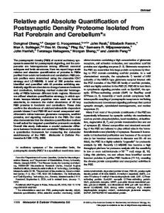
2. EXPERIMENT AND METHOD 2.1 Measurement setup An object to be measured has to be reflective, and in approximate shape of a plane. The object is to be placed as a reflector in one arm of Michelson interferometer, Fig. 1a. In the other arm a reference flat is used. After combining both beams behind a beam splitter, an objective lens performs imaging from the object plane to the plane of image sensor (camera chip). The setup has been focused so that rays deflected by the object shall be focused onto the image sensor. The reference flat is somewhat displaced from zero OPD, thus making a clearly distinguishable absolute offset. For the signal formation and processing we have chosen frequency-scanning interferometry (FSI1 ). The reasons were mainly: (1.) easy and cheap temperature (or current) tuning of contemporary diode lasers; (2.) ability to replace phase shifters by scanning frequency only; (3.) ability to resolve n2π ambiguity, and also we presumed (4.) the method will be more resistant to etalon fringes and superimposed false interference. Our expectation Corresponding author: Marek Peca, [email protected]
a)
b)
0.05
0.00
−0.05
−0.15
−0.30 −0.10
0.15
−0.05
0.20
0.25
0.45
0.50
OptoCad (v 0.94a)
Figure 1. (a) Interferometer layout; (b) drawing of measured object.
of (4.) is based on fact, that spurious fringes resulting from different OPDs in system will generate in turn different fringe density in FSI, which shall be close to orthogonal to the desired OPD for wide frequency scans. As a tunable laser source, 3 DFB diode lasers have been employed, ∼ 2 MHz Lorentzian linewidth, ∆λ ≈ 1.5 nm of temperature tuning range. The nominal center frequencies of these DFB lasers were: 773 nm, 785 nm, 852 nm. The DFB lasers were operated at constant current, variable temperature control. All of them were coupled and multiplexed to a single-mode fiber, illuminating the interferometer through a beam collimator. A part of the fiber light has been tapped off and led to a wavemeter in order to provide accurate actual frequency measurements. The declared accuracy of the wavelenght measurement is 5 × 10⁻⁷ . The camera is based on a 12-bit, APS image sensor, 6 × 6µm pixels. All the optical components were off-the-shelf items: beam splitter cube made of 25.4 mm N-BK7, and a f = 75 mm achromatic doublet made of N-BAF10, N-SF6HT. The system has been set up on an air-suspended breadboard table, and covered under a cardboard box as a rudimentary means of temperature and air flow control.
2.2 Signal processing At each pixel, a dependence of intensity on laser frequency is sampled at several discrete points, see idealized and exaggerated plot in Fig. 2. The intensity function of ideal interferometer, having exactly one path difference (two arms, no spurious reflections), uniform power, no instrumental noise etc., is: I(L, ν) ∝ cos 2π
L 2π + IDC = cos Lν + IDC . λ c
(1)
In our task ν is known variable and the OPD L is a parameter to be estimated. The intensity I(L) as a function of OPD is a cosine waveform with zero phase at zero OPD, as well as at (hypothetical) zero laser frequency. The ultimate goal of absolute FSI is to reconstruct the cosine from sparse measured samples – ideally the waveform shall be extrapolated to origin (ν = 0) with phase error not exceeding π. Otherwise the integer ambiguity n2π can hardly be detected from the data. The L effectively plays a role of fringe repetition rate during the ν sweep.
I(L,ν)
ν1
ν2
ν3
ν Figure 2. Illustration of FSI data sampled at distinct frequency bands.
Within our setup, we have few (three) narrow ν bands, separated by comparatively large gaps. Let us suppose we wish to extrapolate the waveform between two distant bands centered around ν1,2 . We need to have an initial ˆ 0 , and estimated fringe phase at the two exact frequencies: ϕˆ1,2 ≈ ϕ1,2 = (2π/c)Lν1,2 . fringe rate estimate L ˆ 0 = L + εL , ϕˆ1,2 = ϕ1,2 + εϕ . The linear We must take into account the errors of all three prior estimates: L 1,2 extrapolation of phase can be only successful when the errors combined do not exceed ±π: 2π |εL ||ν2 − ν1 | + |εϕ1 | + |εϕ2 | < π. c
(2)
In practice εϕ1,2 will be negligible compared to εL , therefore the prerequisite for extrapolation over ν1 . . . ν2 gap is: |εL |