ABSTRACT Adaptive Methods for the Helmholtz Equation with ...

ABSTRACT Adaptive Methods for the Helmholtz Equation with Discontinuous Coefficients at an Interface James W. Rogers, Jr., Ph.D. Advisor: Qin Sheng, Ph.D. In this dissertation, we explore highly efficient and accurate finite difference methods for the numerical solution of variable coefficient partial differential equations arising in electromagnetic wave applications. We are particularly interested in the Helmholtz equation due to its importance in laser beam propagation simulations. The single lens environments we consider involve physical domains with subregions of differing indices of refraction. Coefficient values possess jump discontinuities at the interface between subregions. We construct novel numerical solution methods that avoid computational instability and maintain high accuracy near the interface. The first class of difference methods developed transforms the differential equation problem to a new boundary value problem for which a numerical solution can be readily computed on rectangular subregions with constant wavenumbers. The second class of numerical methods implemented combines adaptive domain transformation with coefficient smoothing to yield a boundary value problem well-suited for numerical solution on a uniform grid in the computational space. The resulting finite difference schemes do not have treat the grid points near the interface as a special case. A novel matrix analysis technique is implemented to examine the stability of these new methods. Computational verifications are carried out.

Adaptive Methods for the Helmholtz Equation with Discontinuous Coefficients at an Interface by James W. Rogers, Jr., B.S. A Dissertation Approved by the Department of Mathematics

Lance L. Littlejohn, Ph.D., Chairperson Submitted to the Graduate Faculty of Baylor University in Partial Fulfillment of the Requirements for the Degree of Doctor of Philosophy

Approved by the Dissertation Committee

Qin Sheng, Ph.D., Chairperson

John M. Davis, Ph.D.

Johnny L. Henderson, Ph.D.

Klaus Kirsten, Ph.D.

Ian A. Gravagne, Ph.D. Accepted by the Graduate School December 2007

J. Larry Lyon, Ph.D., Dean

Page bearing signatures is kept on file in the Graduate School.

c 2007 by James W. Rogers, Jr. Copyright ° All rights reserved

TABLE OF CONTENTS LIST OF FIGURES

vi

ACKNOWLEDGMENTS

vii

1 Introduction

1

1.1

Interface Problems . . . . . . . . . . . . . . . . . . . . . . . . . . . .

1

1.2

Paraxial Wave Optics . . . . . . . . . . . . . . . . . . . . . . . . . . .

1

1.2.1

The Helmholtz Equation . . . . . . . . . . . . . . . . . . . . .

2

1.2.2

Initial and Boundary Conditions . . . . . . . . . . . . . . . . .

5

Adaptive Grids . . . . . . . . . . . . . . . . . . . . . . . . . . . . . .

7

1.3.1

Uniform Cartesian Grids . . . . . . . . . . . . . . . . . . . . .

8

1.3.2

Uniform Grid Numerical Methods . . . . . . . . . . . . . . . .

9

1.3.3

Goals of an Adaptive Method . . . . . . . . . . . . . . . . . .

11

1.3

2 A Six-Point, Two-Level Finite Difference Scheme

13

2.1

Derivation . . . . . . . . . . . . . . . . . . . . . . . . . . . . . . . . .

13

2.2

Consistency . . . . . . . . . . . . . . . . . . . . . . . . . . . . . . . .

17

2.3

A Stability Analysis Method . . . . . . . . . . . . . . . . . . . . . . .

21

2.4

Homogeneous Paraxial Helmholtz Scheme . . . . . . . . . . . . . . .

26

2.5

Stability of Homogeneous Paraxial Helmholtz Scheme . . . . . . . . .

27

2.6

Coefficient Smoothing . . . . . . . . . . . . . . . . . . . . . . . . . .

30

2.7

Stability of Smoothed Case . . . . . . . . . . . . . . . . . . . . . . . .

33

3 z-Stretching Domain Transformation

36

3.1

Stretching in the z direction . . . . . . . . . . . . . . . . . . . . . . .

36

3.2

z-Stretching Stability . . . . . . . . . . . . . . . . . . . . . . . . . . .

41

iii

3.3

z-Stretching Scheme with Cross Derivative Term . . . . . . . . . . . .

42

3.4

Stability of z-Stretching scheme with Cross Derivative Term . . . . .

46

3.5

Numerical Results . . . . . . . . . . . . . . . . . . . . . . . . . . . . .

49

4 Moving Mesh Methods

53

4.1

Stretching in the r Direction . . . . . . . . . . . . . . . . . . . . . . .

53

4.2

Stability in the Transformed Space . . . . . . . . . . . . . . . . . . .

55

4.3

Adaptive Grid Methods . . . . . . . . . . . . . . . . . . . . . . . . .

57

4.3.1

Adaptive Mesh Refinement . . . . . . . . . . . . . . . . . . . .

57

4.3.2

Grid Redistribution . . . . . . . . . . . . . . . . . . . . . . . .

59

4.4

A Mesh Generator . . . . . . . . . . . . . . . . . . . . . . . . . . . .

60

4.5

A Moving Mesh Method . . . . . . . . . . . . . . . . . . . . . . . . .

63

4.6

A Simple Example . . . . . . . . . . . . . . . . . . . . . . . . . . . .

66

5 The Immersed Interface Method

69

5.1

Jump Conditions . . . . . . . . . . . . . . . . . . . . . . . . . . . . .

70

5.2

Difference Schemes for Irregular Points . . . . . . . . . . . . . . . . .

72

6 Summary

80

6.1

Thesis Contribution . . . . . . . . . . . . . . . . . . . . . . . . . . . .

80

6.2

Future Research . . . . . . . . . . . . . . . . . . . . . . . . . . . . . .

81

6.2.1

The Matrix Analysis Method . . . . . . . . . . . . . . . . . .

81

6.2.2

A Moving Mesh Method for Higher Spatial Dimensions . . . .

83

6.2.3

A Solution Adaptive Moving Mesh Method . . . . . . . . . . .

84

APPENDICES A Derivative and Antiderivative Approximations on Nonuniform Grids A.1 The Delta and Nabla Derivatives . . . . . . . . . . . . . . . . . . . . iv

86 88

A.2 The Diamond-α Dynamic Derivative . . . . . . . . . . . . . . . . . .

91

A.3 A Diamond-α Integral . . . . . . . . . . . . . . . . . . . . . . . . . .

98

A.4 Numerical Examples . . . . . . . . . . . . . . . . . . . . . . . . . . . 100 B Matlab Code

105

B.1 Example r-Stretching Transformations . . . . . . . . . . . . . . . . . 105 B.2 Moving Mesh Method

. . . . . . . . . . . . . . . . . . . . . . . . . . 108

BIBLIOGRAPHY

117

v

LIST OF FIGURES 1.1

The domain. . . . . . . . . . . . . . . . . . . . . . . . . . . . . . . . .

1.2

Discontinuous coefficients can cause inaccuracy and nonphysical oscil-

6

lation. . . . . . . . . . . . . . . . . . . . . . . . . . . . . . . . . . . .

7

2.1

³ ´ Neighborhood of reference point zn− 1 , rm . . . . . . . . . . . . . . .

13

2.2

Simulation with discontinuous coefficient. . . . . . . . . . . . . . . . .

30

3.1

An in-lens domain before and after z-stretching. . . . . . . . . . . . .

41

3.2

z-stretch simulation: intensity of the computed solution near the z-axis. 50

3.3

Normalized intensity graph of experimental data. . . . . . . . . . . .

3.4

z-stretch simulation: real part of the computed solution at the focal

2

50

point. . . . . . . . . . . . . . . . . . . . . . . . . . . . . . . . . . . .

51

3.5

z-stretch simulation: amplitude of real component near the z-axis. . .

51

3.6

z-stretch simulation: amplitude of imaginary component near the z-axis. 52

4.1

The sigma function in r coordinates, and in y coordinates. . . . . . .

64

4.2

The r transformation and derivative with respect to y. . . . . . . . .

65

4.3

Analytic and smoothed coefficient solution, steepness factor β =

.

66

4.4

Solution, β = 12 , in r-stretched and original coordinates. . . . . . . . .

67

4.5

Error β =

4.6

Solution with steep σ, β = 2, no r-stretching, and error due to instability. 68

5.1

Case 1. The interface does not divide points on the right. . . . . . . .

73

5.2

Case 2. Points on right column of stencil divided, with rj−1 < η < rj .

74

5.3

Case 3. Points on right column of stencil divided, with rj < η < rj+1 .

75

5.4

Case 4. Interface exactly divides right column of stencil, η = rj . . . .

76

1 , 10

1 . 10

no r-stretching, and error β = 2, with r-stretching. . . .

vi

67

ACKNOWLEDGMENTS I would like to thank my advisor Qin Sheng for his invaluable insight and direction throughout the dissertation process, and I look forward to continuing our collaboration long into the future. I am very grateful to Johnny Henderson for the crucial support, encouragement, and excellent instruction he provided me during my time at Baylor University. I would also like to express my appreciation to Brian Raines for a unique assistantship opportunity he made available to me, to the members of my committee for their time and effort, and to all of the Baylor mathematics professors and instructors from whom I learned so much. The interaction with my fellow graduate students, especially Curtis Kunkel and Mariette Maroun, has been a valuable resource to me during my graduate studies. In addition, this work has been supported in part by research grants from Baylor University Offices as well as General Dynamics Information Technology and the U.S. Air Force.

vii

CHAPTER ONE Introduction 1.1 Interface Problems Interface problems are boundary value problems where the partial differential equation has one or more coefficients that are discontinuous at some internal curve or surface, called an interface. These type of problems arise when modeling a wide variety of physical processes, such as heat conduction through layers of materials with differing thermal conductivities, magnetic imaging of tissue structures with regions of differing magnetic permeability, geophysical electromagnetic surveying, and multiphase fluid flow in petroleum or groundwater reservoirs with sediment layers of differing porosity or permeability [22, 33, 38]. The problem on which we will focus originates in the modeling of a laser beam propagating from air into and out of a single curved lens, air and lens being layers of media with differing indices of refraction. Since many existing strategies for the numerical solution of partial differential equations were developed for equations with smooth or even constant coefficients, interface problems may pose insurmountable difficulties for conventional numerical methods. In particular, the accuracy of derivative approximations can suffer significantly if they are based on a set of points that straddle an interface, and instability can be introduced into the solution procedure if a coefficient of the equation varies too greatly between sample points in a discretization. 1.2

Paraxial Wave Optics

In order to facilitate optical wave modeling, several approximations have traditionally been employed. The global properties of axially symmetric optical systems are described in terms of paraxial or Gaussian optics, where only rays close to and making small angles with the axis of symmetry are considered [73]. The focal point of 1

2 these paraxial rays is referred to as the principle focus of the system, while deviations from the Gaussian image point are classified as abberations. The paraxial approximation is obtained by replacing the trigonometric functions sine, cosine and tangent by the first term of their Taylor expansions, i.e. sin θ = θ, cos θ = 1, and tan θ = θ. For the equation of motion of electromagnetic waves in a linear homogeneous medium, the substitution results in a wave equation approximation that is parabolic in form. Parabolic wave equation approximations are employed in a number of applications, including acoustics, seismology, geophysical sensing, plasma physics and aerodynamics, microwave signal transmission, as well as optics [17]. Paraxial models are also used extensively in microbeam optoelectronics applications. The approximation is useful both in improving computational efficiency, and reducing the complexity of the model to selectively eliminate certain wave properties, such as reflection [4]. While the paraxial wave approximation is primarily used for modeling waves traveling at small angles to the direction of propagation of the system, several authors have proposed extending it to larger fields and apertures by using higher order differential equations, systems of differential equations, or a generalized set of extended paraxial coordinates [4, 5, 35]. 1.2.1

The Helmholtz Equation Unlike conventional optical light, radiation from lasers is approximately monochro-

matic, with precise phase and amplitude variations in the first-order approximation, and are thus described most accurately by Maxwell’s wave equations [16]. Maxwell’s wave equations are derived from Maxwell’s four field equations, ∇·E=

ρ , ε0

∇ · B = 0,

(1.1) (1.2)

3 ∇×E=−

∂B , ∂t

∇ × B = µ0 J + µ0 ε 0

(1.3) ∂E , ∂t

(1.4)

where E is the electric field, B is the magnetic field, J is the current density, ρ is the electric charge density, ε0 is the permittivity of free space, µ0 is the magnetic permeability of free space, ∇· is the divergence operator, and ∇× is the curl operator. Maxwell’s field equations are coupled first-order differential equations not well suited for use in boundary value problems [56]. For this, we may observe that when the first-order equations are decoupled, we obtain the wave equation, or the timedependent vector Helmholtz equation ∇2 E −

1 ∂2E = 0, c2 ∂t2

where E = E(x, y, z) is the electric field intensity in volts/meter, ∇2 =

∂2 ∂2 ∂2 + + , ∂x2 ∂y 2 ∂z 2

is the Laplacian operator, and c is the phase velocity, or the speed of light in a particular medium. Monochromatic waves can be accurately described by a complex wavefunction U satisfying U (x, y, z, t), = U (x, y, z) exp(i2πνt)

(1.5)

where |U (x, y, z)| and arg (U (x, y, z)) are the amplitude and phase of the wave respectively, ν is the frequency in Hz, and U (x, y, z, t) satisfies the scalar wave equation ∇2 U −

1 ∂2U = 0. c2 ∂t2

(1.6)

By substituting (1.5) into (1.6), we obtain the Helmholtz equation ¡

where k =

¢ ∇2 + k 2 U (x, y, z) = 0,

(1.7)

2π c 2πν = is called the wavenumber. The value λ = is the wavelength. c λ ν

4 Let ϕ(x, y, z) represent the phase of the wavefunction at point (x, y, z). The surfaces of equal phase for the wavefunction, where ϕ(x, y, z) is constant, are called wavefronts. The wavefront normal at (x, y, z) is parallel to the gradient vector ∇ϕ(x, y, z) and represents the direction at which the rate of change of the phase is maximum [57]. We consider wavefunctions with complex amplitudes described by the equation U (x, y, z) = u(x, y, z) exp (−ikz) where i =

√

(1.8)

−1, the complex function u(x, y, z) is called the complex envelope, and

the z axis is taken to be in the direction of the first wavefront normal. If the variation of u(x, y, z) is slow in the z-direction, then we have a wave such that the wavefront normals make small angles with z, a so-called paraxial wave. We substitute (1.8) into the Helmholtz equation (1.7) and factor out exp(−ikz) to obtain ∇2T u(x, y, z) − 2ik

∂u(x, y, z) ∂ 2 u(x, y, z) + = 0, ∂z ∂z 2

(1.9)

where ∇2T

∂2 ∂2 = + ∂x2 ∂y 2

is the transverse Laplacian operator. Because u(x, y, z) varies relatively slowly in the z-direction, for large wavenumbers k we can assume that within a wavelength of the propagation distance, the change in u is small compared to |u| [54]. We have ¯ 2 ¯ ¯∂ u¯ 2 ¯ ¯ ¯ ∂z 2 ¯ ¿ |k u| thus ∂ 2u ≈ 0. ∂z 2 We obtain an approximation of (1.9) ∇2T u(x, y, z) − 2ik

∂u(x, y, z) = 0, ∂z

(1.10)

5 which is called the slowly varying envelope approximation of the Helmholtz equation, or simply the paraxial Helmholtz equation [6, 57]. Next we let 1 y r = (x2 + y 2 ) 2 ≥ 0, φ = arctan . x

Then (1.10) can be written in polar coordinates as µ

∂2 1 ∂2 ∂ 1 ∂ + 2 + 2 2 − 2ik r ∂r ∂r r ∂φ ∂z

¶ u(x, y, z) = 0,

(1.11)

Equation (1.11) is considered sufficiently accurate for laser propagation applications in multi-layer media [30, 31, 66]. In our discussions, we consider the partial differential equation (1.11) in a spherical lens environment. In the case of a cylindrically symmetric domain, we assume ∂2u ≡0 ∂φ2 and simplify the polar paraxial equation (1.11) to yield 1 2ikuz (z, r) = urr (z, r) + ur (z, r). r

(1.12)

Without loss of generality, we may assume that 0 ≤ r ≤ R1 ¿ ∞. 1.2.2

Initial and Boundary Conditions

We employ Neumann boundary conditions ur (z, 0) = ur (z, R1 ) = 0, z > 0,

(1.13)

at the bottom, r = 0 and top, r = R1 of the rectangular domain. For the initial solution of boundary value problem (1.12), (1.13), we use the following approximation of a Gaussian beam with point source [21] µ ¶ r2 1 exp ikz − 2 , u(z, r) = 1 + iZ β (1 + iZ)

(1.14)

6

Figure 1.1. The domain.

where β0 is the Gaussian beam width, while Z, β and A are parameters such that Z=

2z , β 2k

1 1 ik = + , 2 β2 β0 2z0

A = eikz0 .

We also need to know the boundary conditions of the wavefunction at the interface. From Maxwell’s equations and the associated constitutive relations for media, it is possible to show that as a monochromatic wave propagates through media of different refractive indices, its frequency remains the same, but we have the following relations for phase velocity c, wavelength λ and wavenumber k c=

c0 λ0 2π 2πn , λ= , k= = = nk0 n n λ λ0

where c0 , λ0 and k0 are the phase velocity, wavelength and wavenumber in a vacuum and n is the index of refraction of the medium. For our single lens case simulations, we utilize the following high wavenumbers  2πn1   = 9.97543 × 103 , if (z, r) is inside lens area,  k2 = λ k(z, r) =  2πn0 2k1 2   k1 = = = × 9.97543 × 103 , otherwise, λ 3 3 (1.15)

7

0

0

−0.005

−0.005

−0.01 w = imaginary(u)

w = imaginary(u)

−0.01 −0.015 −0.02 −0.025

−0.02

−0.025

−0.03

−0.03

−0.035 −0.04

−0.015

0

0.1

0.2

0.3

0.4 z

0.5

0.6

0.7

0

0.1

0.2

0.3

0.4 z

0.5

0.6

0.7

Figure 1.2: Discontinuous coefficients can cause inaccuracy and nonphysical oscillation. Here we see the mid-lens behavior of the imaginary part of a computed solution of Eq. (1.12) for the case of discontinuous and smoothed wavenumber k functions.

which is reasonably consistent with experimental laser beam wavelengths [30, 32]. Clearly, the coefficient function k(z, r) is discontinuous at the lens interface. Mathematically, relation (1.15) introduces a discontinuity in the coefficient of uz along the boundary between the different media. This adds considerable difficulty to the task of computing the numerical solution of (1.12) [41]. From Maxwell’s equations we can deduce that u(z, r), ur (z, r) and uz (z, r) are continuous across the curved lens boundary [56, 21]. Then examining (1.12), we can see that urr (z, r) will have a jump discontinuity at the interface. These jump conditions will be discussed in detail in Section 5.1. Relation (1.15) represents a single lens situation. We could further consider multiple lens scenarios with additional k values involved. 1.3 Adaptive Grids There are a variety of well established techniques for the numerical solution of boundary value problems, including the widely used finite difference and finite element methods. The majority of these methods depend upon a discrete grid of points upon

8 which an approximate solution of the boundary value problem is computed. The grid must include a sufficient number of points in any local region of the domain to accurately represent the solution. For certain problems, especially interface problems, local regions of high variability, shocks or discontinuities will arise, requiring a very fine grid spacing. If the fine resolution necessary in these regions were to be extended over the entire domain of the problem, the amount of data storage and computational cycles required to compute a solution would be far greater than modern computing devices could provide. Practical considerations then, have driven the development of adaptive grid methods. For the most part, adaptive grid methods fall into two main categories: local grid refinement and grid redistribution [76]. Important early work on local grid refinement was done by Berger and Oliger, who developed the Adaptive Mesh Refinement (AMR) method, a system of successively refined subgrids recursively imposed onto regions of larger, coarser grids [8, 9]. In grid redistribution, often referred to as “moving mesh” methods, the number of points in a grid is fixed, but the positions of these points in the physical space are adjusted via dynamically adaptive transformations so that more points occur in regions where greater accuracy is required. An additional set of differential equations called mesh generators are often solved concurrently with the main problem in order to determine efficient grid transformations [24, 39]. A moving mesh method for finite differences was developed by Dorfi and Drury [19]. We will examine the properties of both types of adaptive grid methods in more detail in later sections. 1.3.1

Uniform Cartesian Grids We wish to employ finite difference methods to find a numerical solution to our

interface problem, and we would like to compute that solution on a uniform Cartesian grid, i.e. a grid with uniform spacings in each spatial coordinate direction. For two-

9 level schemes, uniform spacing is not required in the direction of wave propagation. The advantages of operating on a uniform grid are numerous, with the foremost advantage being the accuracy and simplicity of derivative approximations in such a domain. Examining the Taylor expansion formulas which are the basis for most derivative approximations, we find that when grid spacings are not uniform, we no longer get the cancelation of higher order terms which provides greater order of accuracy for the resulting derivative approximation formulas while using the fewest possible terms. Worse yet, standard difference formulas may not be valid approximations for higher derivatives at all when applied to a nonuniform grid [55, 58]. A uniform grid also facilitates the application of a wide array of well-developed methods, such as fast Poisson solvers and Fast Fourier Transform algorithms, which were originally formulated to use equally spaced sample points [11, 23, 48]. Further, while nonuniform schemes can reduce data array size requirements, this typically comes at the expense of computation time, as well as data space overhead which must be devoted to grid housekeeping. In addition, uniform grid schemes are often much better suited to the optimized vectorization hardware available in modern computer processors, which can provide very significant speed increases for numerical method implementations without the need for specialized programming. 1.3.2

Uniform Grid Numerical Methods Considering the many advantages of uniform Cartesian grids, it is not surpris-

ing that several uniform grid methods have been developed for the numerical solution of partial differential equations with singular or discontinuous coefficients. In 1961, Tikhonov and Samarskii derived second order accurate finite difference approximations of elliptic equations with discontinuous coefficients using Green’s function techniques [70, 72]. Mayo developed fast numerical solution methods for Laplace’s and biharmonic equations with irregular domains by using integral equation formulations to define discontinuous extensions of the equations to regular, embedding domains.

10 The solution of the interface problem thus obtained is computed using fast Poisson solvers on a uniform grid, with correction terms applied to the points adjacent to the interface [48]. Mayo and Greenbaum further developed the technique using parallel algorithms [49]. MacKinnon and Carey, and Fornberg and Meyer-Spasche have also utilized the correction term approach to numerically solve interface problems [47, 25]. One of the most significant and widely utilized uniform grid methods for interface problems is the immersed interface method of Li and LeVeque, which is an extension of the earlier immersed boundary method of Peskin [46, 53]. The central idea of the immersed interface method is to employ a conventional finite difference scheme everywhere on a uniform grid except on “irregular” points, i.e. points which are adjacent to the interface. For the irregular points, modified finite difference equations are derived using the so-called jump relations, which are the relations of the limits of the solution, its derivatives and the coefficient functions as they approach the interface from opposite sides. These jump relations may be obtained from the partial differential equation itself, or by referring to the known behavior of the physical processes being modeled. In the case of an implicit scheme, the modified finite difference equations replace the standard finite difference equations corresponding to the irregular points in the system of equations to be solved. Various authors have adapted and extended the immersed interface method to additional problems. Zhang applied the method to acoustic wave equations across an interface, [78] while Kreiss and Petersson recently proposed a modified version of the immersed interface method to simplify the derivation of the difference equation coefficients at irregular points for two dimensional second order wave equations [40]. While the immersed interface method retains the advantages of a uniform grid and is particularly effective at forcing the computed solution to behave exactly as we want it to near the interface, there are some drawbacks. With the modification of some of the difference equations, a system of equations may lose certain properties,

11 such as diagonal dominance or banded structure, becoming considerably more difficult to solve. For example, a tridiagonal system might lose that structure, and thus no longer be solvable using the simple, efficient Thomas algorithm. Perhaps the biggest disadvantage, however, from an implementation standpoint, is the fact that for each interface problem new difference equations must be derived analytically, depending upon the partial differential equation and jump conditions, as well as the properties, position and orientation of the interface. While this process produces excellent results, it is unlikely that it could ever be automated in software. 1.3.3

Goals of an Adaptive Method We will use domain transformation to map discretization points that are nonuni-

form in the physical space onto a uniform grid in the computational space. A simple example of this technique is used by Shibayama et. al. [66] and is referred to by the authors as a computational space method. In the aforementioned paper, the physical coordinate space (x, z) is mapped onto coordinate space (u, z) by the mapping x = α tan(u) where α is a scaling constant. Here the mapping does not depend on z, the direction of propagation coordinate. In contrast, our moving mesh method will use a transverse direction transformation that is dynamically generated at each propagation step. Our motivation is to produce a numerical method which is flexible enough to adjust to varying interface properties or jump conditions without the need to derive new difference schemes for grid points near the interface. We should not have to determine jump conditions analytically, as long as they are inherent in the partial differential equation and boundary conditions. Ideally, the method should be able to make domain transformation adjustments at a propagation step based solely on the partial differential equation and boundary conditions, the current numerical solution values, and the current dynamically generated transformation function. However, our

12 current study will focus on methods in which domain transformation is based on the shape of the lens domain segment, or on the location of the interface at the grid lines.

CHAPTER TWO A Six-Point, Two-Level Finite Difference Scheme 2.1 Derivation We consider a second-order partial differential equation defined on a domain Ω in the following general form: c4 urr + c3 ur + c2 uz + c1 u + c0 = 0,

(2.1)

where the coefficients ci , 0 ≤ i ≤ 4, are functions of r and z, and the rectangular, two-dimensional domain Ω = {(z, r) | 0 ≤ r ≤ R, 0 ≤ z ≤ Z} for constants R > 0 and Z > 0. Let M, N ∈ Z+ , h =

R Z and τ = . We define a M N

uniform grid of points Ωτ,h = {(mh, nτ ) | 0 ≤ m ≤ M, 0 ≤ n ≤ N } ⊂ Ω.

rm+2 rm+1 rm

(zn−½,rm)

rm−1 rm−2 zn−2

zn−1

zn

Figure 2.1: Neighborhood of reference point grid.

zn+1

zn+2

´ ³ zn− 1 , rm in a uniform (regularly spaced)

13

2

14 Thus M, N are the number of grid points and h, τ are the discretization parameters or step sizes, in the r and z directions respectively. We will use the notation rm = mh and zn = nτ to represent grid line positions in the r and z directions respectively. We write zn− 1 to specify the non-grid point halfway between zn−1 and zn . 2

Definition 2.1. Points in Ω at which partial differential equations and finite difference schemes are evaluated and compared may not be in the set Ωτ,h We call such points reference points. We use the following Taylor expansions to derive approximations for ur , urr , and uz ³ ´ ¡¡ ¢ ¢ 1 at reference point zn− , rm = n − 12 τ, mh : 2

∂u τ ∂u h2 ∂ 2 u τ 2 ∂ 2 u hτ ∂ 2 u h3 ∂ 3 u + + + + + 2 ∂r 2 ∂z 2 ∂r2 8 ∂z 2 2 ∂r∂z 6 ∂r3 2 3 2 3 3 3 4 4 3 4 hτ ∂ u hτ ∂ u τ ∂ u h ∂ u hτ ∂ u + + + + + 2 2 4 ∂r ∂z 8 ∂r∂z 48 ∂z 3 24 ∂r4 12 ∂r3 ∂z 2 2 4 3 4 4 4 ¡ ¢ hτ ∂ u hτ ∂ u τ ∂ u + + + + O(τ 5 ) + O hτ 4 2 2 3 4 16 ∂r ∂z 48 ∂r∂z 384 ∂z ¡ 2 3¢ ¡ 3 2¢ ¡ 4 ¢ ¡ ¢ + O h τ + O h τ + O h τ + O h5 , (2.2)

um+1,n = um,n− 1 + h

τ ∂u τ 2 ∂ 2 u τ 3 ∂ 3 u τ 4 ∂4u + + + + O(τ 5 ), (2.3) 2 2 ∂z 8 ∂z 2 48 ∂z 3 384 ∂z 4 ∂u τ ∂u h2 ∂ 2 u τ 2 ∂ 2 u hτ ∂ 2 u h3 ∂ 3 u + + + − − = um,n− 1 − h 2 ∂r 2 ∂z 2 ∂r2 8 ∂z 2 2 ∂r∂z 6 ∂r3 2 3 3 4 2 3 3 4 4 3 hτ ∂ u hτ ∂ u τ ∂ u h ∂ u hτ ∂ u + − + + − 2 2 4 ∂r ∂z 8 ∂r∂z 48 ∂z 3 24 ∂r4 12 ∂r3 ∂z ¡ 4¢ h2 τ 2 ∂ 4 u hτ 3 ∂ 4 u τ 4 ∂ 4u 5 − + + O(τ ) + O hτ + 16 ∂r2 ∂z 2 48 ∂r∂z 3 384 ∂z 4 ¡ ¢ ¡ ¢ ¡ ¢ ¡ ¢ + O h2 τ 3 + O h3 τ 2 + O h4 τ + O h5 , (2.4)

um,n = um,n− 1 + um−1,n

∂u τ ∂u h2 ∂ 2 u τ 2 ∂ 2 u hτ ∂ 2 u h3 ∂ 3 u − + + − + 2 ∂r 2 ∂z 2 ∂r2 8 ∂z 2 2 ∂r∂z 6 ∂r3 2 3 3 4 4 3 2 3 3 4 hτ ∂ u τ ∂ u h ∂ u hτ ∂ u hτ ∂ u + − + − − 2 2 4 ∂r ∂z 8 ∂r∂z 48 ∂z 3 24 ∂r4 12 ∂r3 ∂z 2 2 3 4 4 4 4 ¡ ¢ hτ ∂ u hτ ∂ u τ ∂ u + − + + O(τ 5 ) + O hτ 4 2 2 3 4 16 ∂r ∂z 48 ∂r∂z 384 ∂z ¡ 2 3¢ ¡ 3 2¢ ¡ 4 ¢ ¡ ¢ + O h τ + O h τ + O h τ + O h5 , (2.5)

um+1,n−1 = um,n− 1 + h

um,n−1 = um,n− 1 − 2

τ 4 ∂ 4u τ ∂u τ 2 ∂ 2 u τ 3 ∂ 3 u + − + + O(τ 5 ) 2 ∂z 8 ∂z 2 48 ∂z 3 384 ∂z 4

(2.6)

15

∂u τ ∂u h2 ∂ 2 u τ 2 ∂ 2 u hτ ∂ 2 u h3 ∂ 3 u + + − + − 2 ∂r 2 ∂z 2 ∂r2 8 ∂z 2 2 ∂r∂z 6 ∂r3 3 2 3 3 3 4 4 3 4 2 hτ ∂ u hτ ∂ u τ ∂ u h ∂ u hτ ∂ u − − + + − 4 ∂r2 ∂z 8 ∂r∂z 2 48 ∂z 3 24 ∂r4 12 ∂r3 ∂z 2 2 4 3 4 4 4 ¡ ¢ hτ ∂ u hτ ∂ u τ ∂ u + + + + O(τ 5 ) + O hτ 4 2 2 3 4 16 ∂r ∂z 48 ∂r∂z 384 ∂z ¡ 2 3¢ ¡ 3 2¢ ¡ 4 ¢ ¡ ¢ + O h τ + O h τ + O h τ + O h5 . (2.7)

um−1,n−1 = um,n− 1 − h

It follows that ½ ¾ 1 um+1,n − um−1,n um+1,n−1 − um−1,n−1 + 2 2h 2h ½ ¾ 3 3 ¡ 5¢ ¡ 3 2¢ ¡ 4¢ 1 ∂u 2h ∂ u hτ 2 ∂ 3 u = 4h + + + O h + O h τ + O hτ 4h ∂r 3 ∂r3 2 ∂r∂z 2 ¡ 4¢ ¡ 2 2¢ ¡ 4¢ ∂u h2 ∂ 3 u τ 2 ∂ 3 u = + + + O h + O h τ + O τ ∂r 6 ∂r3 8 ∂r∂z 2 ¡ ¢ ¡ ¢ ¡ ¢ ∂u = + O h2 + O h2 τ 2 + O τ 2 , ½ ∂r ¾ 1 um+1,n − 2um,n + um−1,n um+1,n−1 − 2um,n−1 + um−1,n−1 + 2 h2 h2 ½ ¾ 2 4 4 4 2 2 ¡ 6¢ ¡ 2 4¢ ¡ 4 2¢ 1 h ∂ u hτ ∂ u 2∂ u = 2 2h + + +O h +O h τ +O h τ 2h ∂r2 6 ∂r4 4 ∂r2 ∂z 2 ¡ ¢ ¡ ¢ ¡ ¢ ∂ 2u = 2 + O h2 + O h2 τ 2 + O τ 2 , ∂r ½ ¾ ¡ 5¢ ¡ ¢ um,n − um,n−1 1 ∂u τ 3 ∂ 3 u ∂u = τ + +O τ = + O τ2 3 τ τ ∂z 24 ∂z ∂z and 1 1 {um,n + um,n−1 } = 2 2

½ 2um,n− 1 2

¡ 6¢ τ 2 ∂ 2u τ 4 ∂ 4u + + + O τ 4 ∂z 2 192 ∂z 4

¾

¡ ¢ = um,n− 1 + O τ 2 . 2

Thus we have ¾ um+1,n − um−1,n um+1,n−1 − um−1,n−1 + 2h 2h ¡ 2¢ ¡ 2 2¢ ¡ 2¢ +O h +O h τ +O τ , (2.8) ¾ ½ 1 um+1,n − 2um,n + um−1,n um+1,n−1 − 2um,n−1 + um−1,n−1 + urr (zn− 1 , rm ) = 2 2 h2 h2 ¢ ¡ ¢ ¡ ¡ ¢ (2.9) + O h2 + O h2 τ 2 + O τ 2 , 1 ur (zn− 1 , rm ) = 2 2

½

16 ¡ ¢ um,n − um,n−1 + O τ2 , (2.10) 2 τ ¡ ¢ 1 u(zn− 1 , rm ) = {um,n + um,n−1 } + O τ 2 , (2.11) 2 2 ³ ´ where all derivatives are evaluated at non-grid point zn− 1 , rm . When τ ≤ Ch for uz (zn− 1 , rm ) =

2

some constant C, we have ½ ¾ ¡ ¢ 1 um+1,n − um−1,n um+1,n−1 − um−1,n−1 ur (zn− 1 , rm ) = + + O h2 , (2.12) 2 2 2h 2h ½ ¾ 1 um+1,n − 2um,n + um−1,n um+1,n−1 − 2um,n−1 + um−1,n−1 + urr (zn− 1 , rm ) = 2 2 h2 h2 ¡ ¢ + O h2 . (2.13) Substituting the approximations (2.8)-(2.11) into Equation (2.1) yields a six-point, two-level, Crank-Nicholson type scheme c4 [um+1,n − 2um,n + um−1,n + um+1,n−1 − 2um,n−1 + um−1,n−1 ] 2h2 c3 + [um+1,n − um−1,n + um+1,n−1 − um−1,n−1 ] 4h c2 c1 + [um,n − um,n−1 ] + [um,n + um,n−1 ] + c0 = 0. τ 2

(2.14)

To facilitate stability and consistency analysis, we rewrite (2.14) in the following implicit form ³ c ³ c ³ c c3 ´ c2 c1 ´ c3 ´ 4 4 4 + u + − + + u + − um−1,n m+1,n m,n 2h2 4h h2 τ 2 2h2 4h ³c ³ c ³ c c3 ´ c2 c1 ´ c3 ´ 4 4 4 =− + um+1,n−1 + 2 + − um,n−1 − − um−1,n−1 + c0 . 2h2 4h h τ 2 2h2 4h (2.15) Next, we will derive additional finite difference approximations for the Neumann boundary conditions ur (z, 0) = 0 and ur (z, R1 ) = 0. We have ur (z, 0) =

¡ ¢ u1,n − u−1,n + O h2 = 0. 2h

Then u−1,n = u1,n + O (h) .

(2.16)

17 We consider the finite difference scheme (2.15) at the boundary r = 0 ³ c ³ c ³ c c3 ´ c2 c1 ´ c3 ´ 4 4 4 + u + − + + u + − u−1,n 1,n 0,n 2h2 4h h2 τ 2 2h2 4h ³ c ³c ³ c c3 ´ c2 c1 ´ c3 ´ 4 4 4 =− + u + + − u − − u−1,n−1 + c0 . 1,n−1 0,n−1 2h2 4h h2 τ 2 2h2 4h Substituting (2.16) into the above, we obtain ³ c c4 c2 c1 ´ 4 u1,n + − 2 + + u0,n h2 h τ 2 ³ c4 c2 c1 ´ c4 = − 2 u1,n−1 + 2 + − u0,n−1 + c0 . h h τ 2

(2.17)

Similarly, at r = R1 we have ur (z, R1 ) =

¡ ¢ uM +1,n − uM −1,n + O h2 = 0, 2h

thus uM +1,n = uM −1,n + O (h) .

(2.18)

We consider the finite difference scheme (2.15) at the boundary r = R1 ³ c ³ c ³ c c3 ´ c2 c1 ´ c3 ´ 4 4 4 + u + − + + u + − uM −1,n M +1,n M,n 2h2 4h h2 τ 2 2h2 4h ³c ³ c ³ c c3 ´ c2 c1 ´ c3 ´ 4 4 4 + u + + − u − − uM −1,n−1 + c0 . =− M +1,n−1 M,n−1 2h2 4h h2 τ 2 2h2 4h Substituting (2.18) into the above, we obtain ³ c c4 c2 c1 ´ 4 uM +1,n + − 2 + + uM,n h2 h τ 2 ³ c4 c4 c2 c1 ´ = − 2 uM +1,n−1 + 2 + − uM,n−1 + c0 . h h τ 2

(2.19)

2.2 Consistency Definition 2.2. We say that the finite difference equation Pτ,h v = f is consistent with the partial differential equation P u = f if for any smooth function φ(z, r) Pτ,h φ − P φ → 0 as τ, h → 0, the convergence being pointwise at each reference point (z, r).

18 Usage of the term “truncation error” can vary somewhat according to source material. The fundamental idea is to provide a measure of the extent to which an exact solution of a differential equation fails to satisfy a difference equation. In this dissertation we will utilize definitions convenient for a Crank-Nicholson type scheme. Definition 2.3. Let φ(z, r) be a smooth function. Then the difference Pτ,h φ−P φ, where Pτ,h φ and P φ are evaluated on reference point (z, r), is called the local truncation error of finite difference scheme Pτ,h v = 0 with respect to partial differential equation P u = 0. Definition 2.4. A scheme Pτ,h v = 0 is accurate of order p in the z direction and q in the r direction if for any smooth function φ(z, r), Pτ,h φ − P φ = O (τ p ) + O (hq ) ,

(2.20)

where Pτ,h φ and differential equation P φ are evaluated at reference point (z, r). We say that the scheme has local order of accuracy (p, q). Recall (2.1). For the theorems and remarks to follow, let P be the linear differential operator such that P u = c4 urr + c3 ur + c2 uz + c1 u + c0

(2.21)

where ci , 0 ≤ i ≤ 4, are functions of r and z. Further, let Pτ,h be the difference operator Pτ,h u =

³ c ³ c ³ c c3 ´ c2 c1 ´ c3 ´ 4 4 4 + u + − + + u + − um−1,n m+1,n m,n 2h2 4h h2 τ 2 2h2 4h ³ c ³ c ³ c c3 ´ c2 c1 ´ c3 ´ 4 4 4 + + u + − − + u + − um−1,n−1 m+1,n−1 m,n−1 2h2 4h h2 τ 2 2h2 4h + c0 ,

(2.22)

where h and τ are the grid step-sizes, m and n the grid indices for the r and z directions, respectively.

19 Theorem 2.1. The finite difference equation Pτ,h v = 0 has a local truncation error of order O (τ 2 ) + O (h2 ) with respect to P u = 0. Proof. Let u(z, r) be a smooth function. By substituting the Taylor expansions (2.2)(2.7) into (2.22) and gathering terms, we see that · 2 ¸ ¡ 4¢ ¡ 2 2¢ ¡ 4¢ ∂ u h2 ∂ 4 u τ 2 ∂ 4 u Pτ,h u = c4 + + +O h +O h τ +O τ ∂r2 12 ∂r4 8 ∂r2 ∂z 2 ¸ · ¡ 4¢ ¡ 2 2¢ ¡ 4¢ ∂u h2 ∂ 3 u τ 2 ∂ 3 u + + +O h +O h τ +O τ + c3 ∂r 6 ∂r3 8 ∂r∂z 2 · ¸ · ¸ ¡ 4¢ ¡ 6¢ τ 2 ∂2u ∂u τ 2 ∂ 3 u τ 4 ∂ 4u + c2 + +O τ + c1 um,n− 1 + + +O τ + c0 2 ∂z 24 ∂z 3 8 ∂z 2 384 ∂z 4 · 2 4 ¸ ∂2u ∂u ∂u h ∂ u τ 2 ∂ 4u = c4 2 + c3 + c2 + c1 um,n− 1 + c0 + c4 + 2 ∂r ∂r ∂z 12 ∂r4 8 ∂r2 ∂z 2 ¸ · ¸ · ¸ · 2 3 ¡ 4¢ τ 2 ∂3u τ 2 ∂ 2u h ∂ u τ 2 ∂3u + + c + c + O h + c3 2 1 6 ∂r3 8 ∂r∂z 2 24 ∂z 3 8 ∂z 2 ¡ ¢ ¡ ¢ + O h2 τ 2 + O τ 4 · 2 4 ¸ ¸ · 2 3 · 2 3 ¸ h ∂ u τ 2 ∂ 4u h ∂ u τ 2 ∂ 3u τ ∂ u = P u + c4 + + c3 + + c2 4 2 2 3 2 12 ∂r 8 ∂r ∂z 6 ∂r 8 ∂r∂z 24 ∂z 3 · 2 2 ¸ ¡ ¢ ¡ ¢ ¡ ¢ τ ∂ u + c1 + O h4 + O h2 τ 2 + O τ 4 . 2 8 ∂z Thus the truncation error ¸ ¸ · 2 4 · 2 3 · 2 3 ¸ h ∂ u τ 2 ∂ 4u h ∂ u τ 2 ∂ 3u τ ∂ u Pτ,h u − P u = c4 + + c + + c 3 2 12 ∂r4 8 ∂r2 ∂z 2 6 ∂r3 8 ∂r∂z 2 24 ∂z 3 · 2 2 ¸ ¡ 4¢ ¡ 2 2¢ ¡ 4¢ τ ∂ u + c1 + O h + O h τ + O τ 8 ∂z 2 ¡ ¢ ¡ ¢ = O τ 2 + O h2 . This completes our proof. Corollary 2.1. The scheme Pτ,h v = 0 has local order of accuracy (2, 2). Proof. By Theorem 2.1, ¡ ¢ ¡ ¢ Pτ,h u − P u = O τ 2 + O h2 . Thus Pτ,h v = 0 has local order of accuracy (2, 2) with respect to P u = O.

20 Theorem 2.2. The scheme Pτ,h v = 0 is consistent with differential equation P u = 0. Proof. By Theorem 2.1 ¡ ¢ ¡ ¢ Pτ,h u − P u = O τ 2 + O h2 → 0 as τ, h → 0. Thus the scheme Pτ,h v = 0 is consistent with differential equation P u = 0. Now let Qτ,h be the difference operator such that ³c ³ c ³c ch,3 ´ ch,2 ch,1 ´ ch,3 ´ h,4 h,4 h,4 Qτ,h u = + um+1,n + − 2 + + um,n + − um−1,n 2h2 4h h τ 2 2h2 4h ³c ´ ³ ´ ch,4 ch,2 ch,1 ch,3 h,4 + + um+1,n−1 + − 2 − + um,n−1 2 2h 4h h τ 2 ³c ch,3 ´ h,4 + − um−1,n−1 + ch,0 , 2h2 4h where ch,i , 0 ≤ i ≤ 4, are functions of r, z and h such that ch,i → ci as h → 0, and h and τ are the grid intervals, m and n the grid indices for the r and z directions respectively. Theorem 2.3. The scheme Qτ,h v = 0 has a truncation error of ∂ 2u ∂u ∂u (ch,4 − c4 ) 2 + (ch,3 − c3 ) + (ch,2 − c2 ) ∂r ∂r ∂z ¡ 2¢ ¡ ¢ + (ch,1 − c1 ) um,n− 1 + ch,0 − c0 + O τ + O h2 2

with respect to P u = 0. Proof. Let u(z, r) be a smooth function. By Theorem 2.1, ¡ ¢ ¡ ¢ Pτ,h u − P u = O τ 2 + O h2 . Thus we have Qτ,h u − P u = Qτ,h u − Pτ,h u + Pτ,h u − P u ∂ 2u ∂u ∂u + (ch,3 − c3 ) + (ch,2 − c2 ) 2 ∂r ∂r ∂z ¡ 2¢ ¡ 2¢ + (ch,1 − c1 ) um,n− 1 + ch,0 − c0 + O τ + O h . = (ch,4 − c4 )

2

This completes our proof.

21 Theorem 2.4. The scheme Qτ,h v = 0 is consistent with P u = 0. Proof. Let u(z, r) be a smooth function. By Theorem 2.3, ∂ 2u ∂u ∂u + (ch,2 − c2 ) + (ch,3 − c3 ) 2 ∂r ∂r ∂z ¡ 2¢ ¡ 2¢ + (ch,1 − c1 ) um,n− 1 + ch,0 − c0 + O τ + O h .

Qτ,h u − P u = (ch,4 − c4 )

2

Since |ch,i − ci | → 0, 0 ≤ i ≤ 4, as h → 0, we have Qτ,h u − P u → 0 as τ, h → 0. We conclude that Qτ,h v = 0 is consistent with P u = 0.

2.3 A Stability Analysis Method While we were able to demonstrate consistency for the general form of our scheme when the coefficients are taken from any partial differential equation of the form (2.1), stability of the scheme when applied to a specific problem will have to be established for each case. Definition 2.5. A finite difference scheme may be written as a system of linear equations: Bun = Cun−1 , or un = B −1 Cun−1 , M ×M where vector un = {uk,n }M are coefficient k=0 and the difference operators B, C ∈ C

matrices. Let E = B −1 C. If there exists a constant K > 0 independent of n, h and τ such that kE n k ≤ K for some norm k · k, we say that the scheme is stable in the Lax-Richtmyer sense [42, 51].

22 In the above definition and in much of the literature, the matrix B −1 C is assumed to be constant with respect to the direction of propagation, in other words, B −1 C is the same at each z-step. However, in several schemes we wish to explore, B −1 C is dependent on z. We must return to the fundamental concepts of stability of an iterative finite difference scheme and formulate a definition of stability suitable for our purposes. Consider a finite difference scheme written in the form un = An un−1 + fn−1 where the right-hand side matrix An can vary with each propagation step. The solution at propagation level n can be obtained by applying the relation recursively to the initial solution u0 , i.e. Ã n ! Ã n ! Ã n ! Y Y Y un = A k u0 + Ak f0 + Ak f1 + . . . + An fn−2 + fn−1 . k=1

k=2

(2.23)

k=3

If we perturb the vector u0 of initial values to u ˜ 0 , the solution at propagation step n will be ! ! Ã n ! Ã n Ã n Y Y Y Ak f1 + . . . + An fn−2 + fn−1 . Ak f0 + Ak u ˜0 + u ñ =

(2.24)

k=3

k=2

k=1

Let en be the error vector at propagation step n defined as en = u ˜ n − un . Then by (2.23) and (2.24), Ã en = u ˜ n − un =

n Y

! Ak

Ã (˜ u0 − u0 ) =

k=1

n Y

! Ak

e0 .

(2.25)

k=1

Let ρ(A) be the spectral radius of matrix A. If ρ(An ) ≤ 1 for all 0 < nτ < Z and any transverse direction step size 0 < h < ² for some ² > 0, Q then k nk=1 Ak k ≤ 1.

23 By (2.25), this stability condition will guarantee that the perturbations will not increase exponentially with n. However, it does not always guarantee convergence. Additional parameter constraints may need to be determined. To facilitate our analysis of the stability of our schemes, some preliminary results concerning matrices must be established. Definition 2.6. An n × n Hermitian matrix A is said to be positive definite if x∗ Ax > 0 , for all nonzero x ∈ Cn . Definition 2.7. An n × n Hermitian matrix A is said to be positive semidefinite if x∗ Ax ≥ 0 , for all nonzero x ∈ Cn . Note: While the definitions of positive definite and positive semidefinite are sometimes extended to include non-Hermitian matrices, we will limit our usage to the Hermitian case, as do Horn and Johnson [36, 37]. Definition 2.8. A matrix A ∈ Cn×n is said to be positive semistable if the real part of every eigenvalue of A is nonnegative. Lemma 2.1. Let A, B, C ∈ Cn×n be such that B = dI + A, C = dI − A, where d ∈ R, d > 0. Then every eigenvector v ∈ Cn of any of the three matrices is also an eigenvector of the other two, i.e. Av = λA v, Bv = λB v and Cv = λC v, for λA , λB , λC ∈ C with the following relationship between the corresponding eigenvalues: λB = d + λA = 2d − λC , λC = d − λA = 2d − λB .

24 Proof. LetA, B, C ∈ Cn×n as above. Clearly, each of the matrices commutes with the other two, and thus by a well known result in matrix theory, they share a common basis of eigenvectors. To show the eigenvalue relations, let v ∈ Cn be an eigenvector of A with corresponding eigenvalue λA , i.e, Av = λA v. Then Cv = (dI − A) v = dIv − Av = dv − λA v = (d − λA ) v and thus λC = d − λA . Also, Bv = (dI + A) v = dIv + Av = dv + λA v = (d + λA ) v and we have λB = d + λA . Theorem 2.5. Let A, B, C ∈ Cn×n be such that B = dI + A, C = dI − A, where d ∈ R, d > 0. Then the difference scheme defined by Bun = Cun−1 is stable if and only if matrix A is positive semistable. Proof. Let A, B, C ∈ Cn×n be such that B = dI + A, C = dI − A, where d ∈ R, d > 0. Then by Lemma 2.1, any eigenvalue λ of the matrix B −1 C is of the form λ=

d − λA , d + λA

where λA is an eigenvalue of A. It follows that |λ| =

4dRe(λA ) |d − λA | (d − Re(λA ))2 + Im2 (λA ) = 1 − . = 2 |d + λA | (d + Re(λA ))2 + Im (λA ) (d + Re(λA ))2 + Im2 (λA )

25 Case 1: Re(λA ) < 0 ¯ ¯ ¯ ¯ 4dRe(λ ) A ¯ > 1. |λ| = 1 + ¯¯ (d + Re(λA ))2 + Im2 (λA ) ¯ Case 2: Re(λA ) = 0 |λ| = 1 +

4d · 0 = 1 + 0 = 1. (d + Re(λA ))2 + Im2 (λA )

Case 3: Re(λA ) > 0 ¯ ¯ ¯ ¯ 4dRe(λ ) A ¯ < 1. |λ| = 1 − ¯¯ (d + Re(λA ))2 + Im2 (λA ) ¯ Thus we see that for an arbitrary eigenvalue λ of B −1 C, |λ| ≤ 1 if and only if the real parts of the eigenvalues of A are nonnegative. Therefore ρ(B −1 C) ≤ 1 if and only if the real parts of all eigenvalues of A are nonnegative. We conclude that our scheme is stable if and only if A is positive semistable. Consider the general form of our six-point, two-level Crank-Nicholson type scheme 2τ (2.15) with c0 = 0. We multiply through by to obtain c2 µ µ ¶¶ τ ³ c4 c3 ´ τ 2c4 c3 ´ τ ³ c4 + u + 2 − − c − um−1,n u + m+1,n 1 m,n c2 h2 2h c2 h2 c2 2h2 4h µ µ ¶¶ c3 ´ τ 2c4 c3 ´ τ ³ c4 τ ³ c4 + u + 2 + − c − um−1,n−1 . =− u − m+1,n−1 1 m,n−1 c2 h2 2h c2 h2 c2 h2 2h This can be expressed in matrix form Bun = Cun−1 with B = 2I + A,

C = 2I − A,

26 and



            A=          

a1

q1

0

···

b2

a2

q2

0

0

b3

a3

q3

··· ··· ··· ···

0

0

···

where τ am = − c2 (z, mh) bm =

µ

bN −1 aN −1 0

bN

0

  ···     0              qN −1    aN

¶ 2c4 (z, mh) − c1 (z, mh) , h2

c4 (z, mh) c3 (z, mh) c4 (z, mh) c3 (z, mh) − , qm = + . 2 2h 4h 2h2 4h

Theorem 2.6. Our six-point, two-level Crank-Nicholson type scheme is stable for a partial differential equation of form (2.1) if and only if the corresponding matrix A as defined above is positive semistable. Proof. It follows immediately from Theorem 2.5.

2.4 Homogeneous Paraxial Helmholtz Scheme We derive a Crank-Nicholson scheme for the paraxial Helmholtz equation for the case of homogeneous media. Recall Equation (1.12), the paraxial Helmholtz equation in a radially symmetric polar domain 1 2ikuz (z, r) = urr (z, r) + ur (z, r). r First, we identify the coefficients of the paraxial Helmholtz equation which correspond to the coefficients c0 through c4 of equation (2.1) given in Section 2.1 1 c4 = 1, c3 = , c2 = −2ik, , c1 = 0, c0 = 0. r

27 Then we substitute these specific coefficients into the implicit form general finite difference scheme (2.15) to obtain µ

¶ µ ¶ µ ¶ 1 1 1 2ik 1 1 − + um+1,n + + um,n − − um−1,n 2h2 4rh h2 τ 2h2 4rh µ ¶ µ ¶ µ ¶ 1 1 1 2ik 1 1 + um+1,n−1 + − 2 + um,n−1 + − um−1,n−1 . (2.26) = 2h2 4rh h τ 2h2 4rh −τ i , we can rewrite this as 2kh2 µ ¶ µ ¶ 1 1 −α 1+ um+1,n + (2 + 2α) um,n − α 1 − um−1,n 2m 2m µ ¶ µ ¶ 1 1 =α 1 + um+1,n−1 + (2 − 2α) um,n−1 + α 1 − um−1,n−1 . 2m 2m

By substituting the relation r = mh and α =

(2.27)

Using the same method as above, we use (2.17) and (2.19) to derive finite difference equations associated with the boundary conditions of our scheme. −2αu1,n + (2 + 2α) u0,n = 2αu1,n−1 + (2 − 2α) u0,n−1 and (2 + 2α) uM,n − 2αuM −1,n = (2 − 2α) uM,n−1 + 2αuM −1,n−1 . 2.5

Stability of Homogeneous Paraxial Helmholtz Scheme

Lemma 2.2. Let A ∈ Rn×n be tridiagonal with all sub and super-diagonal elements positive, or all sub and super-diagonal elements negative. Then there exists a diagonal matrix D such that D−1 AD is a real symmetric matrix.

28 Proof. We proceed as in Smith [67]. Let A ∈ RN ×N such that   0 ··· 0   a1 c1     b a c 0 · · ·   2 2 2      0 b3 a3 c3 0        ···   A=    · · ·         · · ·      · · · 0 bN −1 aN −1 cN −1      0 ··· 0 bN aN where bi > 0, 2 ≤ i ≤ N and ci > 0, 1 ≤ i ≤ N − 1. Let D ∈ CN ×N be a real diagonal matrix with diagonal elements d1 , d2 , ..., dN . Then  c1 d1 0 ···  a1 d2   b2 d2 a c2 d2 0  d1 2 d3   c3 d3  0 b3dd3 a3 d4 2    ···  −1 DAD =   ···     ···    ··· 0 bN d−1Nd−2N −1 aN −1   bN dN 0 ··· 0 dN −1 q Set d1 = 1 and di =

ci−1 di−1 bi

 0 ··· 0

cN −1 dN −1 dN

                     

aN

for 2 ≤ i ≤ N . Since ci−1 and bi have the same sign,

all di will be positive. Then bi di ci−1 di−1 = , 2 ≤ i ≤ N. di di−1 We see that D−1 AD is a real symmetric matrix. For the case of negative off-diagonal elements, substitute −A for A above.

29 Lemma 2.3. Let A ∈ Rn×n be tridiagonal with all sub and super-diagonal elements positive, or all sub and super-diagonal elements negative. Then all eigenvalues of A are real. Proof. Let A be as above. By Lemma 2.2 there exists a diagonal matrix D such that D−1 AD is a real symmetric matrix. Then A is similar to a real symmetric matrix, which has only real eigenvalues. Thus A has only real eigenvalues. Theorem 2.7. Let the wavenumber k be a constant. Then the homogeneous paraxial Helmholtz finite difference scheme is stable. Proof. Let the wavenumber k be a constant. Consider the finite difference scheme (2.27) in matrix form Bun = Cun−1 . We have B = 2I + A, C = 2I − A, and A = αH, where  2 −2 0 ··· 0  ³ ´ ³ ´  1  − 1− 1 2 − 1 + 2(1) 0 ··· 2(1)    ···    H= ···    ···   ³ ´ ³ ´  ··· 0 − 1 − 2(M1−1) 2 − 1 + 2(M1−1)   0 ··· 0 −2 2

          .        

Observe that α is purely imaginary and that matrix H is a real tridiagonal matrix with all off-diagonal elements negative. Then by Lemma 2.3, H has real eigenvalues. Thus A has purely imaginary eigenvalues and is therefore positive semistable. By Theorem 2.5, we can conclude that homogeneous paraxial Helmholtz finite difference scheme is stable.

30

real(u)*real(u)+imag(u)*imag(u)

0.995

0.99

0.985

0.98

0

0.5

1

1.5

z

Figure 2.2: Simulation using the two-level, six-point scheme with discontinuous coefficient: intensity of the computed solution near the z-axis. No focusing is observed.

2.6

Coefficient Smoothing

To facilitate the use of conventional numerical techniques for partial differential equations with discontinuous coefficients at an interface, several methods have been proposed that replace the discontinuous coefficient functions with continuous functions derived through harmonic averaging of the coefficient function values near the interface [2, 14, 72]. We shall explore a somewhat different approach to coefficient function smoothing. The consistency result of Theorem 2.4 implies that we may replace a discontinuous coefficient function ci in a partial differential equation of form (2.1) with a continuous function ch,i of h that approaches ci as h → 0 to derive our scheme and still maintain consistency. However, the truncation error will no longer be O(h2 ), but will now be proportional to max |ch,i −ci | near the interface. Brown demonstrated that for 0≤i≤4

a piecewise continuous wave equation with coefficient functions approximated by continuous functions, the accuracy with which the amplitude is computed is dependent on the accuracy with which the interface conditions are approximated [14].

31 We once again consider Equation (1.12), the paraxial Helmholtz equation in a radially symmetric polar domain 1 2ikuz (z, r) = urr (z, r) + ur (z, r). r Let η(z) =

p

R2 − (z − R)2 be the function which gives the position of the interface

(the point of discontinuity of the wavenumber, k) with respect to the r axis. The k parameter can be expressed as k(z, r) =

   k2 , r < η(z),

(2.28)

  k1 , r ≥ η(z).

We construct a continuous function kh that approximates k, k(z, r) ≈ kh (z, r) = k2 + (k1 − k2 ) σh (z, r),

(2.29)

where σh (z, r) is monotonically increasing with respect to r, σh (z, 0) = 0, σh (z, R1 ) = 1 for 0 ≤ z ≤ Z, and σh (z, r) ≈

   0, r < η(z),   1, r > η(z).

A candidate for our σh function is ³ ´ ³ ´ −η(z) tanh r−η(z) − tanh h h ³ ´ ³ ´, σh (z, r) = −η(z) tanh R1 −η(z) − tanh h h which is the hyperbolic tangent function with a steepness factor of

1 , h

centered at

η(z), and normalized so that σ(z, 0) = 0, σ(z, R1 ) = 1 for 0 ≤ z ≤ Z. Then    0, r < η(z),    1 σlim (z, r) = lim σh (z, r) = , r = η(z), 2 h→0      1, r > η(z). and

(2.30)

32       klim (z, r) = lim kh (z, r) = h→0

k1 ,

r < η(z),

k1 + 21 (k2 − k1 ) , r = η(z),      k2 , r > η(z).

(2.31)

We see that klim (z, r) = k(z, r) except at r = η(z). For convenience, we modify our model by replacing k with klim to obtain 1 2iklim uz (z, r) = urr (z, r) + ur (z, r) r

(2.32)

and further replace klim with kh , to obtain a smoothed-coefficient model from which we will derive a finite difference scheme consistent with (2.32). 1 2ikh uz (z, r) = urr (z, r) + ur (z, r). r

(2.33)

We form the six-point, two-level finite difference scheme with ch,0 = 0, ch,1 = 0, ch,2 = 2ikh , ch,3 = −

1 and ch,4 = −1 r

in implicit form µ ¶ µ ¶ µ ¶ 1 1 1 1 2ikh 1 − + um+1,n + + um,n − − um−1,n 2h2 4rh h2 τ 2h2 4rh µ ¶ µ ¶ µ ¶ 1 1 1 1 2ikh 1 = + um+1,n−1 + − 2 + um,n−1 + − um−1,n−1 2h2 4rh h τ 2h2 4rh (2.34) or on the grid lines r = mh µ ¶ µ ¶ µ ¶ α 1 α α 1 − 1+ um+1,n + 2 + 2 um,n − 1− um−1,n kh 2m kh kh 2m µ ¶ µ ¶ µ ¶ 1 α α 1 α 1+ um+1,n−1 + 2 − 2 um,n−1 + 1− um−1,n−1 = kh 2m kh kh 2m

(2.35)

−τ i . 2h2 As in the homogeneous case, we substitute the specific coefficient ci values into (2.17) where α =

and (2.19) to obtain difference equations for the boundary conditions. At r = 0 we have

µ ¶ µ ¶ α α α α u0,n = 2 u1,n−1 + 2 − 2 u0,n−1 −2 u1,n + 2 + 2 kh kh kh kh

(2.36)

33 and at r = R1 ¶ µ ¶ µ α α α α 2+2 uM,n − 2 uM −1,n = 2 − 2 uM,n−1 + 2 uM −1,n−1 . kh kh kh kh

(2.37)

2.7 Stability of Smoothed Case We need further results concerning matrix properties, especially the eigenvalues of tridiagonal matrices. Definition 2.9. Let A ∈ CN ×N . We define the functions ι+ : C N ×N → Z, ι− : C N ×N → Z and ι0 : C N ×N → Z as follows ι+ (A) : the number of eigenvalues of A, including multiplicities, with positive real part. ι− (A) : the number of eigenvalues of A, including multiplicities, with negative real part. ι0 (A) : the number of eigenvalues of A, including multiplicities, with zero real part. The row vector ι(A) := [ι+ (A), ι− (A), ι0 (A)] is called the inertia of A. Lemma 2.4 (Horn [37]). Let A, B ∈ CN ×N with B Hermitian and A + A∗ positive definite. Then ι(AB) = ι(B). Theorem 2.8. Let A, B ∈ CN ×N with B Hermitian, A diagonal and A + A∗ positive semidefinite. Then ι− (AB) ≤ ι− (B). Proof. Let A, B ∈ CN ×N with B Hermitian, A diagonal and A + A∗ positive semidefinite. We have A + A∗ = diag {2Re(a11 ), 2Re(a22 ), . . . , 2Re(aN N )} , with Re(amm ) ≥ 0, 1 ≤ m ≤ N . Choose real ² > 0. Then Re(amm ) + ² > 0, 1 ≤ m ≤ N and (A + ²I) + (A + ²I)∗ = diag {2Re(a11 ) + 2², 2Re(a22 ) + 2², . . . , 2Re(aN N ) + 2²} .

34 Thus, (A + ²I) + (A + ²I)∗ is positive definite. By Lemma 2.4, it follows that i ((A + ²I)B) = ι(B) for all ² > 0.

(2.38)

Assume ι− (AB) > ι− (B). Since lim(A + ²I)B = AB and eigenvalues are a contin²→0

uous function of the elements of a matrix, there must exist some ²0 > 0 such that ι− ((A + ²I)B) = ι− (AB) > ι− (B) for all ² < ²0 . This contradicts (2.38). Thus ι− (AB) ≤ ι− (B). Theorem 2.9. Let S ∈ CN ×N and H ∈ RN ×N . If (i) S is diagonal; (ii) S + S ∗ is positive semidefinite; (iii) H is tridiagonal with all off-diagonal elements positive or all off-diagonal elements negative, then ι− (SH) ≤ ι− (H). Proof. Let S and H be as above. Then by Theorem 2.2, there exists a diagonal matrix D such that D−1 HD is a real symmetric matrix, thus Hermitian. By Lemma 2.8, ι− (SD−1 HD) ≤ ι− (D−1 HD). Since D−1 and S are diagonal, they commute. Then SD−1 HD = D−1 SHD. Then ι− (SH) = ι− (D−1 SHD) = ι− (SD−1 HD) ≤ ι− (D−1 HD) = ι− (H).

Theorem 2.10. The finite difference scheme (2.35), (2.36), (2.37) is stable. Proof. Consider the finite difference scheme (2.35) in the form of a matrix equation: Bun = Cun−1

35 with B = 2I + A, C = 2I − A, and A = αH, where  2 − k20 0 ··· 0 k0  ´ ³ ´  1 ³ 1 2 1  − − k11 1 + 2(1) 0 ··· k1  k1 1 − 2(1)   ···    H= ···    ···   ³ ´ ³  1 1 1 2 ··· 0 − kM −1 1 − 2(M −1) − kM −1 1 +  kM −1  2 0 ··· 0 − k2M kM

               ´   1  2(M −1) 

with km = kh (mh), for 0 ≤ m ≤ M . As in the case of the homogeneous scheme, α is purely imaginary, and since km > 0 for all 0 ≤ m ≤ M , matrix H is a real tridiagonal matrix with all off-diagonal elements negative. Then by Lemma 2.3, H has real eigenvalues. Thus A has purely imaginary eigenvalues, and is therefore positive semistable. Then by Theorem 2.5, the smoothed coefficient scheme is stable.

CHAPTER THREE z-Stretching Domain Transformation In this chapter we explore domain segmentation and transformation. We first use properties of the solution consistent with the slowly varying envelope approximation to derive an efficient approximation method for our model boundary value problem. Then we examine further applications. 3.1 Stretching in the z direction If the pre-lens, lens and post-lens segments of the domain were successive rectangular areas along the direction of propagation, we would be able to use conventional finite difference techniques to solve the paraxial Helmholtz equation for a constant k on each segment. We could achieve this scenario by ”stretching” each segment by a 1-1 coordinate transformation onto a rectangular area and transforming the partial differential equation for the new coordinate system. By shifting the z-coordinate (propagation direction) values for the points of a domain segment, while keeping the transverse r-coordinate values constant, we can obtain rectangular subdomains such that the solution computed at the rightmost edge of each segment would become the initial condition of the next segment. We will call this type of transformation z-stretching. We are looking for a solution of the form u(x(z, r), y(z, r)) which satisfies the boundary value problem 1 2ikuz (x(z, r), y(z, r)) = urr (x(z, r), y(z, r)) + ur (x(z, r), y(z, r)), r ur (x(z, 0), y(z, 0)) = 0, ur (x(z, R1 ), y(z, R1 )) = 0. 36

37 We find the derivatives with respect to the transformed coordinates ∂u ∂u ∂y ∂u ∂x = + , ∂r ∂y ∂r ∂x ∂r ∂u ∂u ∂y ∂u ∂x = + , ∂z ∂y ∂z ∂x ∂z µ ¶2 µ ¶2 ∂ 2u ∂u ∂ 2 y ∂ 2 u ∂y ∂ 2 u ∂y ∂x ∂u ∂ 2 x ∂ 2 u ∂x = + + + +2 . ∂r2 ∂y ∂r2 ∂y 2 ∂r ∂y∂x ∂r ∂r ∂x ∂r2 ∂x2 ∂r Our transformed partial differential equation is µ 2ik

∂u ∂y ∂u ∂x + ∂y ∂z ∂x ∂z

¶

∂u ∂ 2 x ∂ 2 u + + ∂x ∂r2 ∂x2

∂u ∂ 2 y ∂ 2 u = + ∂y ∂r2 ∂y 2 µ

∂x ∂r

¶2

1 + r

µ

µ

∂y ∂r

¶2 +2

∂ 2 u ∂y ∂x ∂y∂x ∂r ∂r

∂u ∂y ∂u ∂x + ∂y ∂r ∂x ∂r

¶ .

Collecting terms we can write the above as µ

¶ µ ¶ ∂x ∂ 2 x 1 ∂x ∂y ∂ 2 y 1 ∂y 2ik − 2 − ux = −2ik + + uy ∂z ∂r r ∂r ∂z ∂r2 r ∂r µ ¶ µ ¶2 µ ¶2 ∂y ∂x ∂x ∂y uyy + 2 uyx + uxx . + ∂r ∂r ∂r ∂r

(3.1)

In this method, rather than derive a difference scheme for the pre-lens segment we will evaluate the input beam equation at the lens surface and use this as the initial solution for the simulation of the lens segment. The solution at the right edge of the lens segment becomes the initial solution of the post-lens segment, which we simulate using the homogeneous scheme described earlier. We wish to map the lens area Ω : 0 ≤ z ≤ Z, (z − R)2 + r2 ≤ R2 , r ≥ 0, onto the rectangular area Ω1 : 0 ≤ x ≤ Z, 0 ≤ y ≤ R1 using z-stretching. A natural choice is the following one-to-one transformation √ ¢ ¡ z − R − R2 − r 2 √ ¢Z, y(z, r) = r, ¡ x(z, r) = Z − R − R2 − r 2 with inverse transformation z(x, y) = R −

p

R2 − y 2 +

³ í p xh Z − R − R2 − y 2 , r(x, y) = y. Z

38 We have ∂y ∂ 2y ∂y = 1, = 0, = 0, 2 ∂r ∂r ∂z ∂x rZ (z − Z) =√ √ ¡ ¡ ¢¢2 , ∂r R2 − r 2 Z − R − R2 − r 2 √ √ ¡ ¡ ¢ ¢ Z −R3 + Z + R2 − r2 R2 + 2r2 R2 − r2 (Z − z) ∂ 2x =− , √ ¡ ¡ ¢¢3 ∂r2 (R2 − r2 )3/2 Z − R − R2 − r2 and

³ ∂x Z ∂z y x´ √ ¡ ¢, = =√ 1− . ∂z ∂y Z Z − R − R2 − r 2 R2 − r 2 We define functions

∂x (x − Z) y h ³ í , (r (x, y) , z (x, y)) = p p ∂r 2 2 2 2 R −y Z − R− R −y h i p 3 2 − y 2 (R2 + 2y 2 ) − Z (x − Z) R − R 2 ∂ x ψ(x, y) := 2 (r (x, y) , z (x, y)) = í2 , h ³ p 3 ∂r 2 2 2 2 2 (R − y ) Z − R − R − y φ(x, y) :=

θ(x, y) :=

∂x Z ³ ´. (r (x, y) , z (x, y)) = p ∂z Z − R − R2 − y 2

Equation (3.1) becomes µ

¶ 1 1 2ikθ − ψ − φ ux = uy + uyy + 2φuxy + φ2 uxx . y y

(3.2)

Theorem 3.1. The slowly varying envelope approximation implies that the term φ2 uxx in (3.2) is negligible. Proof. For a fixed value of y in the transformed lens segment, |uxx | is bounded by the value of |uxx | at x = 0. Equivalently in the physical space, for a fixed value of r, √ |uxx | is bounded by the value of |uxx | at the lens surface z = R − R2 − r2 . Clearly, |uxx | is monotonically increasing with respect to y. Because we are stretching along the direction of propagation, we have the relation √ ¡ ¡ ¢¢ Z − R − R2 − r 2 uxx = uzz , Z

39 where the derivative term on the left is evaluated at a point in the computational space, and the derivative term on the right is evaluated at the corresponding point in the physical space. We find that R12 Z ³ ´´ |uzz | φ |uxx | ≤ p 2 2 2 2 (R − R1 ) Z − R − R − R1 2

³

for all points in the lens segment. Thus in a typical lens where the slowly varying envelope approximation is applicable, neglecting φ2 uxx , the last term on the righthand side of equation (3.2), will not decrease the accuracy of the approximation. Solely for the purpose of analysis, we will first assume that the cross derivative uzr is also negligible. With this assumption, by a similar argument to above we can demonstrate that the term 2φuxy is negligible as well. Within the lens segment, our transformed equation can be simplified to µ ¶ 1 1 2ikθ − ψ − φ ux = uy + uyy . y y

(3.3)

The coefficients of our simplified equation are µ ¶ 1 1 c4 = 1, c3 = , c2 = − 2ikθ − ψ − φ , c1 = 0, c0 = 0. y y Substituting the specific coefficient ci values into (2.15) we obtain the scheme ¶ µ · ¸¶ 1 1 1 1 1 + um+1,n + − 2 − 2ikθ − ψ − φ um,n 2h2 4hy h τ y µ ¶ µ ¶ 1 1 1 1 − + + um−1,n = − um+1,n−1 2h2 4hy 2h2 4hy µ ¸¶ µ · ¶ 1 1 1 1 1 + − − 2ikθ − ψ − φ um,n−1 − um−1,n−1 . h2 τ y 2h2 4hy µ

On the grid lines y = mh, we can write the above as µ

1 −αγ 1 + 2m

¶

µ

1 um+1,n + (2 + 2αγ) um,n − αγ 1 − 2m

¶ um−1,n

40 µ

1 = αγ 1 + 2m

¶

µ

1 um+1,n−1 + (2 − 2αγ) um,n−1 + αγ 1 − 2m

¶ um−1,n−1

where α=

τ 1 , γ(x, y) = . h2 2ikθ − ψ − y1 φ

For the boundary condition at y = 0 and y = R1 we have

uy (x, 0) = uz zy (x, 0) + ur ry (x, 0) = uz · 0 + ur (x, 0) = 0, and uy (x, R1 ) = uz zy (x, R1 ) + ur ry (x, R1 ) = uz · 0 + ur (x, R1 ) = 0. Substituting the specific coefficient values into the general form for the boundary value difference equations, we obtain −2αγu1,n + (2 + 2αγ) u0,n = 2αγu1,n−1 + (2 − 2αγ) u0,n−1 , and (2 + 2αγ) uM,n − 2αγuM −1,n = (2 − 2αγ) uM,n−1 + 2αγuM −1,n−1 . It is interesting to note that for a lens that tapers to a point at the top, the geometric interpretation of this new boundary condition is that the single point (Z, R1 ) has been stretched into the upper edge of our transformed rectangular domain, i.e. the upper boundary in the computational space corresponds to the single point (Z, R1 ) in the physical space. Expressing the scheme in matrix form Bun = Cun−1 , we have B = 2I + A,

C = 2I − A,

41

R1

r

y

R1

0

Z

0

Z

z

x

Figure 3.1: LEFT: An in-lens domain before z-stretching. RIGHT: The in-lens domain after z-stretching.

where 

2αγ0 −2αγ0 1 −αγ1 (1+ 2(1) ) 2αγ1  ···

A= 

··· 0

0 1 −αγ1 (1− 2(1) ) ··· −αγM −1 (1+ 2(M1−1) ) 0

0 ···

3.2

··· 0

0 ···

  .

 ··· 2αγM −1 −αγM −1 (1− 2(M1−1) ) −2αγM 2αγM

z-Stretching Stability

Theorem 3.2. Let xzr ≈ 0. Then the z-stretched scheme is stable Proof. For the z-stretched scheme, we have A = αSH, where α > 0,   2 −2 0 ··· 0  γ0 0 ··· 1 1 −(1+ 2(1) ··· ) 2 −(1− 2(1) ) 0 0 γ1 0   ···  , S =  ··· ··· ··· H=   ··· ··· 0 γM −1 ··· 0 −(1+ 2(M1−1) ) 2 −(1− 2(M1−1) ) 0 ··· 0 0

···

0

−2

2

0 ···

 

0 γM

Looking at H row-wise, we see that the Gershgorin circles are centered at 2, and have radius 2. Thus the eigenvalues of H are located on the closed right half of the complex plane, i.e. the real parts of the eigenvalues are non-negative. Subsequently,

42 we have γ(x, y) =

³

1

´

1 φ(x, y) y

2ikθ(x, y) − ψ(x, y) + ´ ³ − ψ(x, y) + y1 φ(x, y) − 2ikθ(x, y) =³ . ´2 2 1 ψ(x, y) + y φ(x, y) + (2kθ(x, y))

Now we examine the terms of the γ function, beginning with    −Z(Z−x) < 0, 0 ≤ x < Z, RZ 2 . ψ(x, 0) =   0, x=Z q With respect to y, ψ(x, y) changes sign at asymptote y = R2 − (R − Z)2 = R1 . We find that ψ(x, y) < 0 for 0 ≤ y < R1 , 0 ≤ x < Z. Next, we have    −(Z−x) < 0, 0 ≤ x < Z, 1 RZ . φ(x, 0) =  y  0, x=Z Examining φ, we find that φ(x, y) < 0 for 0 ≤ y < R1 , 0 ≤ x < Z. Thus we can see that ³ ´ − ψ(x, y) + y1 φ(x, y) ≥ 0, for 0 ≤ y < R1 , 0 ≤ x < Z. Re (γ(x, y)) = ³ ´2 ψ(x, y) + y1 φ(x, y) + (2kθ(x, y))2 Thus matrix S is positive semidefinite. Consequently by Theorem 2.9, ι− (αHS) = ι− (HS) ≤ ι− (H) = 0. Thus A is positive semistable and we can conclude that the z-stretched scheme is stable.

3.3

z-Stretching Scheme with Cross Derivative Term

We now discard the assumption that the cross derivative term in the transformed equation (3.2) is negligible. It will be necessary therefore to establish a few results concerning partial differential equations of the form c5 uzr + c4 urr + c3 ur + c2 uz + c1 u + c0 = 0,

(3.4)

43 where ci , 0 ≤ i ≤ 5 are functions of r and z. For the theorems and remarks to follow, let P be the differential operator such that P u = c5 uzr + c4 urr + c3 ur + c2 uz + c1 u + c0 . (3.5) ³ ´ We use the Taylor expansions (2.2)-(2.7) around reference point zn− 1 , rm to derive 2 ½ ¾ 1 um+1,n − um−1,n um+1,n−1 − um−1,n−1 uzr = − + O(h2 ). (3.6) τ 2h 2h We substitute the approximations (2.8)-(2.11) and (3.6) into equation (3.4) to form a six-point, two-level difference scheme as follows c5 [um+1,n − um−1,n − um+1,n−1 + um−1,n−1 ] 2τ h c4 + 2 [um+1,n − 2um,n + um−1,n + um+1,n−1 − 2um,n−1 + um−1,n−1 ] 2h c3 [um+1,n − um−1,n + um+1,n−1 − um−1,n−1 ] + 4h c2 c1 + [um,n − um,n−1 ] + [um,n + um,n−1 ] + c0 = 0. τ 2 The above can be expressed as a difference operator in implicit form ³ c ³ c c4 c3 ´ c2 c1 ´ 5 4 Pτ,h u = um+1,n + − 2 + + um,n + 2+ 2hτ 2h 4h h τ 2 ³ c c4 c3 ´ 5 + − um−1,n + 2− 2hτ 2h 4h ³ c ³c c4 c3 ´ c2 c1 ´ 5 4 =− − + 2+ um+1,n−1 + 2 + − um,n−1 2hτ 2h 4h h τ 2 ³ c c4 c3 ´ 5 − + 2− um−1,n−1 + c0 2hτ 2h 4h

(3.7)

where h and τ are the grid step-sizes, m and n the grid indices for the r and z directions respectively. For the Neumann boundary conditions ur (0) = 0, ur (R1 ) = 0 as in Section 2.1 we derive difference equations in general form ³ c c2 c1 ´ c4 4 u + − + + u0,n 1,n h2 h2 τ 2 ³c c4 c2 c1 ´ 4 = − 2 u1,n−1 + 2 + − u0,n−1 + c0 h h τ 2

(3.8)

44 and ³ c c4 c2 c1 ´ 4 uM −1,n + − 2 + + uM,n h2 h τ 2 ³ c4 c2 c1 ´ c4 = − 2 uM −1,n−1 + 2 + − uM,n−1 + c0 . h h τ 2

(3.9)

Theorem 3.3. The scheme Pτ,h v = 0 has a local truncation error of order O (τ 2 ) + O (h2 ) with respect to P u = 0. Proof. Let u(z, r) be a smooth function. By substituting the Taylor expansions (2.2)(2.7) into (3.7) and gathering terms, we see that ·

¸ ¡ 4¢ ¡ 2 2¢ ¡ 4¢ ∂ 2u h2 ∂ 4 u τ 2 ∂4u Pτ,h u = c5 + + +O h +O h τ +O τ ∂z∂r 6 ∂z∂r3 24 ∂z 3 ∂r ¸ · 2 ¡ 4¢ ¡ 2 2¢ ¡ 4¢ ∂ u h2 ∂ 4 u τ 2 ∂ 4 u + + +O h +O h τ +O τ + c4 ∂r2 12 ∂r4 8 ∂r2 ∂z 2 ¸ · ¡ 4¢ ¡ 2 2¢ ¡ 4¢ ∂u h2 ∂ 3 u τ 2 ∂ 3 u + + +O h +O h τ +O τ + c3 ∂r 6 ∂r3 8 ∂r∂z 2 · ¸ ¸ · ¡ 4¢ ¡ 6¢ ∂u τ 2 ∂ 3 u τ 2 ∂ 2u τ 4 ∂ 4u + c2 + +O τ + c1 um,n− 1 + + +O τ + c0 2 ∂z 24 ∂z 3 8 ∂z 2 384 ∂z 4 ∂2u ∂u ∂u ∂ 2u + c4 2 + c3 + c2 + c1 um,n− 1 + c0 = c5 2 ∂z∂r ∂z· ¸ ¸ · 2 4 ∂r 2 ∂r 4 2 4 h ∂ u τ ∂ u h ∂ u τ 2 ∂4u + c5 + + c4 + 6 ∂z∂r3 24 ∂z 3 ∂r 12 ∂r4 8 ∂r2 ∂z 2 · 2 3 ¸ ¸ · · 2 2 ¸ ¡ 4¢ h ∂ u τ 2 ∂ 3u τ 2 ∂ 3u τ ∂ u + c3 + + c + c + O h 2 1 6 ∂r3 8 ∂r∂z 2 24 ∂z 3 8 ∂z 2 ¡ ¢ ¡ ¢ + O h2 τ 2 + O τ 4 ¸ ¸ · 2 4 · 2 4 h ∂ u τ 2 ∂ 4u h ∂ u τ 2 ∂4u = P u + c5 + + c4 + 6 ∂z∂r3 24 ∂z 3 ∂r 12 ∂r4 8 ∂r2 ∂z 2 · 2 3 · · ¸ ¸ ¸ ¡ ¢ h ∂ u τ 2 ∂ 3u τ 2 ∂ 3u τ 2 ∂ 2u + c3 + + c2 + c1 + O h4 3 2 3 2 6 ∂r 8 ∂r∂z 24 ∂z 8 ∂z ¢ ¡ ¢ ¡ + O h2 τ 2 + O τ 4 .

45 Thus the truncation error · 2 4 · 2 4 ¸ ¸ h ∂ u h ∂ u τ 2 ∂ 4u τ 2 ∂ 4u Pτ,h − P u = c5 + + c4 + 6 ∂z∂r3 24 ∂z 3 ∂r 12 ∂r4 8 ∂r2 ∂z 2 · 2 3 ¸ · ¸ · 2 2 ¸ h ∂ u τ 2 ∂3u τ 2 ∂3u τ ∂ u + c3 + + c2 + c1 3 2 3 6 ∂r 8 ∂r∂z 24 ∂z 8 ∂z 2 ¡ ¢ ¡ ¢ ¡ ¢ ¡ ¢ ¡ ¢ + O h4 + O h2 τ 2 + O τ 4 = O τ 2 + O h2 . This completes our proof. Corollary 3.1. The scheme Pτ,h v = 0 has local order of accuracy (2, 2). Proof. By Theorem 3.3, ¡ ¢ ¡ ¢ Pτ,h − P u = O τ 2 + O h2 . Thus Pτ,h v = 0 has local order of accuracy (2, 2) with respect to P u = O. Theorem 3.4. The scheme Pτ,h v = 0 is consistent with differential equation P u = 0. Proof. By Theorem 3.3 ¡ ¢ ¡ ¢ Pτ,h − P u = O τ 2 + O h2 → 0 as τ, h → 0. Thus the scheme Pτ,h v = 0 is consistent with differential equation P u = 0. With a non-negligible cross derivative term, our transformed equation (3.2) becomes

µ

¶ 1 1 2ikθ − ψ − φ ux = uy + uyy + 2φuxy . y y

The coefficients of our simplified equation with cross derivative term are µ ¶ 1 1 c5 = 2φ, c4 = 1, c3 = , c2 = − 2ikθ − ψ − φ , c1 = 0, c0 = 0. y y Substituting the specific coefficient ci values into (3.7) we obtain the scheme µ ¸¶ ¶ µ · 2φ 1 1 1 1 1 + 2+ um+1,n + − 2 − 2ikθ − ψ − φ um,n 2hτ 2h 4hy h τ y

(3.10)

46 µ

¶ µ ¶ 2φ 1 1 2φ 1 1 + − + 2− um−1,n = − − + 2+ um+1,n−1 2hτ 2h 4hy 2hτ 2h 4hy µ · ¸¶ µ ¶ 1 1 1 2φ 1 1 − 2ikθ − ψ − φ um,n−1 − um−1,n−1 . + + 2− h2 τ y 2hτ 2h 4hy On the grid lines y = mh, we can write the above as µ ¶¸ µ ¶¸ · 1 2φ 1 2φ +α 1+ −γ um+1,n + (2 + 2αγ)um,n − γ − + α 1 − um−1,n h 2m h 2m ¶¸ · µ 2φ 1 um+1,n−1 + (2 − 2αγ)um,n−1 =γ − +α 1+ h 2m · ¶¸ µ 2φ 1 +γ um−1,n−1 (3.11) +α 1− h 2m ·

where α=

τ 1 , γ(x, y) = . 2 h 2ikθ − ψ − y1 φ

Substituting the specific coefficient values into the general form for the boundary value difference equations, we obtain −2αγu1,n + (2 + 2αγ) u0,n = 2αγu1,n−1 + (2 − 2αγ) u0,n−1 , and (2 + 2αγ) uM,n − 2αγuM −1,n = (2 − 2αγ) uM,n−1 + 2αγuM −1,n−1 . 3.4 Stability of z-Stretching scheme with Cross Derivative Term To determine the stability of the z-stretching scheme with the cross derivative term, we will need to establish additional lemmas concerning matrices. Lemma 3.1. Let A ∈ Cn×n be nonsingular. Then A + A∗ is positive definite if and ∗

only if A−1 + (A−1 ) is positive definite. Proof. Let A ∈ Cn×n such that A is nonsingular and A + A∗ is positive definite. Then x∗ (A + A∗ ) x > 0 , for all nonzero x ∈ Cn .

47 Let x ∈ Cn . Since A is nonsingular, ∃y ∈ Cn such that x = Ay. Then ¡ ¡ ¢∗ ¢ ¡ ¢∗ x∗ A−1 + A−1 x = x∗ A−1 x + x∗ A−1 x ¡ ¢∗ = (Ay)∗ A−1 Ay + (Ay)∗ A−1 Ay = y∗ A∗ y + y∗ A∗ (A∗ )−1 Ay = y∗ A∗ y + y∗ Ay = y∗ (A + A∗ ) y > 0.

Lemma 3.2. Let A, B ∈ Cn×n with A positive semistable and B nonsingular. Further assume B + B ∗ is positive definite. Then AB −1 is positive semistable. Proof. Let A, B ∈ Cn×n with A positive semistable, B nonsingular, and B + B ∗ ∗

positive definite. By Lemma 3.1, B −1 + (B −1 ) is positive definite. By Lemma 2.4, ι (AB −1 ) = ι (A) . Thus AB −1 is positive semistable. Theorem 3.5. Let A, B, C, G ∈ Cn×n be such that G is nonsingular and B = G + A, C = G − A. Then the difference scheme defined by Bun = Cun−1 is stable if and only if AG−1 is positive semistable. e C, e G ∈ Cn×n be such that G is nonsingular and Proof. Let A, B, C, B, e = I + AG−1 , C e = I − AG−1 B = G + A, C = G − A, B e −1 C. e Specifically We note that the matrix B −1 C is similar to the matrix B ¡ ¢ G B −1 C G−1 = G (G + A)−1 (G − A) G−1 ¢−1 ¡ (G − A) G−1 = (G + A)G−1 ¢ ¢−1 ¡ ¡ e e −1 C. I − AG−1 = B = I + AG−1

48 e −1 C), e and we see that the difference scheme defined by Then ρ(B −1 C) = ρ(B Bun = Cun−1 is stable if and only if the scheme e n = Cu e n−1 Bu is stable. Thus the conclusion follows from Theorem 2.5. Theorem 3.6. Let Re (γ (x, y)) ≥ 0 for 0 ≤ y < R1 and ¯ ¯ ¯ 2γ (x, y) φ (x, y) ¯ ¯ ¯ < 1 for 0 ≤ y < R1 , 0 ≤ x < Z. ¯ ¯ h Then scheme (3.11) is stable. Proof. Let Re (γ (x, y)) ≥ 0 for 0 ≤ y < R1 and ¯ ¯ ¯ 2γ (x, y) φ (x, y) ¯ ¯ ¯ < 1 for 0 ≤ y < R1 , 0 ≤ x < Z. ¯ ¯ h Expressing scheme (3.11) in matrix form Bun = Cun−1 we have B = (G + A) , C = (G − A) where matrix A is the same as in the z-stretching with no cross derivative scheme, and



 2

0

  γφ − 1 1 2  h   ···    G=       0  ···  0 ···

0

···

γ1 φ1 h

0

··· ··· − γM −1hφM −1

2

0

0

0

  ···              γM −1 φM −1   h  2

49 where γm = γ(x, mh) and φm = γ(x, mh). Then 

 2   γφ − 1 1  h      ∗ G+G =        ···  0

− γ1hφ1

0 γ1 φ1 h

2

−

··· γ2 φ2 h

0

··· ··· ··· γM −2 φM −2 h

0 ···

−

γM −1 φM −1 h

0

2 γM −1 φM −1 h

0

   ···       .      γM −1 φM −1   h  2

We will apply Sylvester’s Criterion, which states that a Hermitian matrix A is positive definite if and only if all principal minors of A have a positive determinate [26]. For a tridiagonal matrix, we observe that the determinates of the principle minors can be expressed in recursive form as so det [A]{k,...,n} = an,n det [A]{k,...,n−1} − an,n−1 an−1,n det [A]{k,...,n−2} . With our assumptions it is straightforward to demonstrate via induction that all principal minors have positive determinate. Thus G + G∗ is positive definite. We demonstrated in the previous case that A is positive semistable, thus by Lemma 3.2, AG−1 is positive semistable. Then by Theorem 3.5, we see that our scheme is stable.

3.5

Numerical Results

Simulation results were obtained using the z-stretching method with crossderivative term included. Within the lens segment, the grid utilized 5,000 points in the transverse y-direction and 32,000 points in the x-direction of propagation. The function (1.14) approximating a Gaussian beam with point source was used as the initial value, with point source located at z0 = 10 cm., and beam width β0 = 1.5 cm.

50 4

x 10 12

10

I = v2 + w2

8

6

4

2

2.3

2.4

2.5

2.6

2.7

2.8

2.9

3

3.1

3.2

z

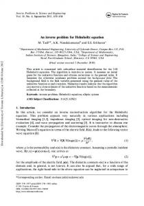
Figure 3.2: z-stretch simulation: intensity of the computed solution near the z-axis, at r = h.

The post-peak oscillation in the graph of the solution intensity near the z-axis matches behavior observed in experimental data.

Figure 3.3. Normalized intensity graph of experimental data.

51

350 300 250

u

200 150 100 50 0 −50 0

0.5

1

1.5

r

Figure 3.4: z-stretch simulation: real part of the computed solution at the focal point z = 2.74 cm.

300

v = real(u)

200

100

0

−100

−200 2.4

2.6

2.8

3

3.2 z

3.4

3.6

3.8

4

Figure 3.5: z-stretch simulation: amplitude of the real part of the computed solution near the z-axis, at r = h.

52

250 200 150

w = imaginary(u)

100 50 0 −50 −100 −150 −200 −250 2.4

2.6

2.8

3

3.2 z

3.4

3.6

3.8

4

Figure 3.6: z-stretch simulation: amplitude of the imaginary part of the computed solution near the z-axis, at r = h.

CHAPTER FOUR Moving Mesh Methods 4.1 Stretching in the r Direction We next consider stretching only in the transverse r direction. It will be convenient in this case to formulate our transformation in terms of the mappings from the computational space to the physical space, r = r(x, y) and z = x. We see that ∂z ∂ 2z ∂z ∂ 2z = 1, = 0, = 0, = 0. ∂x ∂x2 ∂y ∂y 2 We first derive the transformed derivatives ∂u ∂u ∂z ∂u ∂r ∂u ∂u ∂r = + = + , ∂x ∂z ∂x ∂r ∂x ∂z ∂r ∂x ∂u ∂u ∂z ∂u ∂r ∂u ∂r = + = , ∂y ∂z ∂y ∂r ∂y ∂r ∂y µ 2 µ ¶ ¶ ∂ u ∂z ∂ 2 u ∂r ∂r ∂u ∂ 2 r ∂u ∂r ∂ 2u = = + + ∂y 2 ∂r ∂y y ∂z∂r ∂y ∂r2 ∂y ∂y ∂r ∂y 2 µ 2 ¶ µ ¶2 ∂ u ∂r ∂r ∂u ∂ 2 r ∂ 2 u ∂r ∂u ∂ 2 r = + = 2 + . ∂r2 ∂y ∂y ∂r ∂y 2 ∂r ∂y ∂r ∂y 2 Isolating the derivatives in the physical space, we find µ ¶ rx uyy ry − uy ryy 1 uz = ux − uy , ur = uy , urr = . ry ry ry3 Substituting the above into Equation (3.1), we obtain the transformed partial differential equation · 2ik ux − uy

µ

rx ry

¶¸ =

uyy ry − uy ryy 1 + uy . 3 ry rry

Collecting derivative terms we can rewrite this as µ ¶ 1 ryy 1 2ikry ux = uyy + 2ikrx − 2 + uy . ry ry r The transformation function r has the properties that r(0) = 0, r(R1 ) = R1 , ry (0) > 0, ry (R1 ) > 0. 53

(4.1)

54 Then the relation ∂u ∂u ∂z ∂u ∂r ∂u ∂r = + = ∂y ∂z ∂y ∂r ∂y ∂r ∂y implies the transformed boundary conditions ∂u ∂u (0) = 0, (R1 ) = 0. ∂y ∂y Next, we define a finite difference scheme by the method described in Section 2.1. Our coefficients are ch,0 = 0, ch,1 = 0, ch,2 = −2ikh ry , ch,3 = 2ikh rx −

ryy 1 1 + , ch,4 = . 2 ry r ry

(4.2)

Substituting these coefficients into (2.15), we obtain the scheme · ¸¶ µ ¶ 1 1 ryy 1 1 2ikh ry + 2ikh rx − 2 + um+1,n + − 2 − um,n 2h2 ry 4h ry r h ry τ · ¸¶ µ 1 1 ryy 1 − 2ikh rx − 2 + um−1,n + 2h2 ry 4h ry r µ · ¸¶ µ ¶ 1 1 1 ryy 1 2ikh ry = − + 2ikh rx − 2 + um+1,n−1 + − um,n−1 2h2 ry 4h ry r h2 ry τ · ¸¶ µ 1 1 ryy 1 − 2ikh rx − 2 + um−1,n−1 . − 2h2 ry 4h ry r µ

τ , we rewrite the above as 2h2 · ¸¶ µ ¶ µ iα ryy 1 2iα hry 1+ 2ikh rx − 2 + um+1,n + − + 2 um,n kh ry2 2 ry r kh ry2 µ · ¸¶ iα hry ryy 1 + 1− 2ikh rx − 2 + um−1,n kh ry2 2 ry r µ · ¸¶ µ ¶ iα hry ryy 1 2iα 1+ + 2 um,n−1 =− 2ikh rx − 2 + um+1,n−1 + kh ry2 2 ry r kh ry2 µ · ¸¶ iα hry ryy 1 − 1− 2ikrx − 2 + um−1,n−1 . (4.3) kh ry2 2 ry r

Setting α =

We likewise substitute the specific coefficient ci values into (2.17) and (2.19) to form the difference equations for the boundary conditions. µ ¶ µ ¶ 2iα 2iα 2iα 2iα u1,n + − + 2 u0,n = − u1,n−1 + + 2 u0,n−1 kh ry2 kh ry2 kh ry2 kh ry2

(4.4)

55 and µ

¶ µ ¶ 2iα 2iα 2iα 2iα + 2 uM,n + uM −1,n = + 2 uM,n−1 − uM −1,n−1 . − 2 2 2 kh r y kh ry kh ry kh ry2

(4.5)

Theorem 4.1. The scheme (4.3) has truncation error ¡ ¢ ¡ ¢ 2i (kh − k) (ry ux − rx uy ) + O τ 2 + O h2 . with respect to the transformed equation (4.1). Proof. By Theorem 2.3, the truncation error is ∂u ∂ 2u ∂u + (ch,3 − c3 ) + (ch,2 − c2 ) 2 ∂y ∂y ∂x ¡ 2¢ ¡ ¢ + (ch,1 − c1 ) um,n− 1 + ch,0 − c0 + O τ + O h2

(ch,4 − c4 )

2

Substituting the specific coefficients (4.2) into the above, we obtain a truncation error of ¡ ¢ ¡ ¢ 2i (kh − k) (ry ux − rx uy ) + O τ 2 + O h2 .

4.2 Stability in the Transformed Space Theorem 4.2. Let H ∈ CM ×M be  −2   1 − θ1       H=        ···  0

such that  2

0

−2

1 + θ1

··· ···

0

1 − θM −1

···

0

···

0

  0 ···        ,    ···    −2 1 + θM −1   2 −2

56 where

· ¸ hry (mh) ryy (mh) 1 θm = 2ikh (mh)rx (mh) − 2 + 2 ry (mh) r(mh)

and r is the r-stretching transformation r = r(x, y). Then the difference scheme (4.3), (4.4), (4.5) is stable if and only if the matrix iH is positive semistable. Proof. We can express the scheme (4.3), (4.4), (4.5) in matrix form Bun = Cun−1 with

α=

τ , h2

B = 2I + A,   ϕ0 0   0 ϕ 1    ···  S=     · · · 0   0 ···

C = 2I − A, A = iαSH,  ··· 0   0 ···     1  , ϕm = ,  2 (mh) k (mh)r h y  ···   ϕM −1 0    0 ϕM

and H is as above. By Theorem 2.5, the scheme is stable if and only if A is positive semistable. Since kh (y) > 0, ry (y) > 0, for all 0 ≤ y ≤ R1 , S is positive definite. Also, α > 0, therefore αS is positive definite. Thus A = (αS)(iH) is positive semistable if and only if iH is positive semistable. Definition 4.1. A refinement path is a sequence of mesh sizes τ and h, both of which tend to zero. We typically specify a relationship between τ and h, for example, τ ≤ Ch for some constant C, as a constraint on the refinement path. For the r-stretching method, as h → 0, the transform function and derivatives are dependent on h. To evaluate stability, we have the following theorem.

57 Theorem 4.3. We assume a constraint on the refinement path of τ ≤ Ch for some constant C. Let the transform function, r(x, y, h), and derivatives of the r-stretching method be such that |θm | → 0, as h → 0, for all 0 ≤ m ≤ M − 1. Then the eigenvalues of iH approach pure imaginary as h → 0. Proof. As h → 0, H → H0 where  −2 2 0    1 −2 1    ···    H0 =  ···       1 · · · 0  0 ··· 0

 ···

0

  0 · · ·       .    ···    −2 1   2 −2

Since the subdiagonal and superdiagonal entries of H0 are all positive reals, by Lemma 2.3, the eigenvalues of H0 are real. Eigenvalues are a continuous function of the coefficients of a matrix, thus the eigenvalues of iH approach pure imaginary as h → 0.

4.3 Adaptive Grid Methods We will examine previous adaptive grid methods in greater detail, to determine what ideas and methods we can apply to our adaptive techniques. 4.3.1

Adaptive Mesh Refinement Berger and Oliger introduced the Adaptive Mesh Refinement (AMR) method in

1984, originally applied to hyperbolic partial differential equations [8]. The technique

58 proceeds as follows: A base grid consisting of one or more component meshes of points with uniform spacing in each coordinate direction and with sufficient resolution for those regions of least variability in the solution is constructed for the entire domain. During computation, smaller subgrids are placed in regions of greater variability. These subgrids are rectangular, possibly rotated with respect to the base grid, and have a finer mesh with uniform grid spacings in each coordinate direction that have the same relative ratios as the grid spacings in the base grid. The points of the mesh of a subgrid do not have to line up with the points of the base grid in any way. Initial and boundary values for the subgrid are obtained through interpolation from the values calculated on the coarser grid, and a separate solution is then computed for the grid with these boundary values. If the subgrid is rotated with respect to the base grid, the difference equations are transformed onto the rotated coordinates. Successively finer subgrids may be placed on top subgrids recursively. To generate subgrids, truncation error for points on a coarse grid are estimated using a Richardson extrapolation and a finer subgrid is placed to cover each region where the error estimate is greater than a determined tolerance. Refinement is by an arbitrary even integer ratio, which in numerical examples is typically chosen to be four [10]. Rotation is used if it is desirable that a feature of the solution should be normal or tangent to a coordinate direction. If for some area within a subgrid, error estimates are still too high, finer subgrids are applied in a nested hierarchy. The Adaptive Mesh Refinement method was applied to several one and two dimensional shock problems and compared to simulations using uniform meshes with the resolution of the finest subgrid. Considerable savings were achieved in computation time and storage requirement, with error estimates being comparable, or in some cases better due to rotation of the subgrids [8].

59 4.3.2

Grid Redistribution Grid redistribution or “moving mesh” methods utilize a fixed number of spatial

grid points. These grid points are “moved” within the physical space so that a higher concentration of them occur in regions where, because of some local solution feature such as greater variability, more points are needed to represent the solution accurately. The repositioning of the grid points is achieved via coordinate transformation. Beginning with a uniform grid in a rectangular computational space, a 1-1 mapping is defined from the computational space to the physical space. As the simulation proceeds, the mapping is dynamically adapted to reposition grid points where needed in the physical space at each propagation step. The study of how to define useful mappings is a well-developed field referred to as grid generation or mesh generation [24, 39, 71]. An example mapping would be the widely used transformation of cartesian coordinates into polar, cylindrical or spherical coordinates. Such a transformation from a uniform coordinate system onto a general space corresponds directly to the concept of a general curvilinear coordinate system for the physical space, as used in differential geometry and other fields. Typically, the boundary of the computational space corresponds to the boundary of physical space. Magnifying a particular subregion in a physical domain via coordinate transformation is functionally equivalent to decreasing the grid spacings in that region. The numerical computation occurs on the uniform grid in the computational space, sometimes called the logical space. The partial differential equations to be solved in the physical space must be transformed into the uniform coordinate system. The mapping must possess certain properties for the transformed equations to be valid. Definition 4.2. For a coordinate transformation z = z(x, y), r = r(x, y),

60 the matrix





∂z  ∂x

J=

∂r ∂x

∂z ∂y  ∂r ∂y



is called the Jacobian matrix of the transformation, while the determinate J = |J| is referred to as the Jacobian. The quality of the transformation can be determined by properties of the Jacobian. For instance, for the transformation to be 1-1, the Jacobian must have full rank. Transformations are often designed to distribute some function, called a monitor function evenly throughout the physical domain. Most such techniques are based on the equidistribution principle of de Boor [18]. The calculus of variations is commonly employed to obtain a mesh generating equation. The minimizer of a functional can be used to obtain a partial differential equation which is solved by numerical means to generate transformed grid coordinates. We will use this technique to obtain a mesh generator for our r-stretching method. 4.4

A Mesh Generator

We choose the monitor function g(y) = [r(y) + σr (r(y))]2 = ([1 + σr (r(y))] ry )2 . Our object is to produce a mesh generator that will concentrate up to half of the grid points in the region of the interface, without increasing the spacing by more than a factor of 2 between points away from the interface. Theorem 4.4. For a continuous sigma function σ(r), a unique solution of the initial value problem [1 + R1 σr (r(y))] ry = 2,

(4.6)

r(0) = 0

(4.7)

exists and has the following properties:

61 (i) r(R1 ) = R1 (ii) max(ry ) < 2, 0 ≤ y ≤ R1 (iii) max(R1 σ(y)) = max(R1 σr (r(y)) ry ) < 2, 0 ≤ y ≤ R1 Proof. Let f (r) = y =

1 2

(r + R1 σ(r)) . Our sigma functions are monotonically in-

creasing and σ(0) = 0, σ(R1 ) = 1. Thus f (r) is monotonically increasing, and f (0) = 0, f (R1 ) =

1 (R1 + R1 σ(R1 )) = R1 . 2

Then we have the inverse function r(y) = f −1 (y), which is monotonically increasing, and ry =

1 f0

(f −1 (y))

=

2 . 1 + R1 σr (r(y))

Substituting f −1 (y) into (4.6), we see that it is a solution. (i) We have r(R1 ) = f −1 (R1 ) = R1 . (ii) Assume ry ≥ 2. Then 1 + R1 σr (r(y)) ≤ 1 and therefore R1 σr (r(y)) ≤ 0. Contradicts R1 > 0 and σ(r) monotonically increasing. Thus ry < 2. (iii) Assume R1 σr (r(y)) ry ≥ 2. Then r(y) ≤ 0, which contradicts r(y) monotonically increasing. Thus R1 σr (r(y)) ry < 2.

Theorem 4.5. The solution of (4.6), (4.7) minimizes the functional Z R1 I(r) = (σr (r(y))ry + ry )2 dy 0

Z

R1

=

{[σr (r(y)) + 1] ry }2 dy

0

over the set of admissible functions r(y), such that r(y) ∈ C 2 [0, R1 ], r(0) = 0, r(R1 ) = R1 .

62 Proof. Let I(r) be the functional defined above and c(y) ∈ C 2 [0, R1 ] be a function such that c(0) = c(R1 ) = 0. Then for any ε > 0, the function t(y, ε) = r(y) + εc(y) is admissible. We define a function of ε,

Z

R1

F (ε) =

[(σt (t(y, ε)) + 1) (ry + εcy )]2 dy

0

If r(y) minimizes the functional I(r), we must have a minimum of F (ε) at ε = 0. We examine the derivative Z

R1

0

F (ε) =

2 {[(σt (t(y, ε)) + 1) ty ] [c(y)σtt (t(y, ε))ty + cy (σt (t(y, ε)) + 1)]} dy 0

at ε = 0, Z

R1

0

F (0) =

2 {[(σr (r(y)) + 1) ry ] [c(y)σrr (r(y))ry + cy (σr (r(y)) + 1)]} dy 0

½Z

Z

R1

c(y) [σr (r(y)) +

=2 0

Z

R1

=2 0

Z

R1

−2 0

Z

R1

=2 0

1] σrr (r(y))ry2 dy

¾

R1

+

2

cy [σr (r(y)) + 1] ry 0

c(y) [σr (r(y)) + 1] σrr (r(y))ry2 dy

¡ ¢ c(y) 2 [σr (r(y)) + 1] ry2 σrr(r(y)) + [σr (r(y)) + 1]2

© ª c(y) − [σr (r(y)) + 1] ry2 σrr (r(y)) + [σr (r(y)) + 1]2 ryy dy = 0.

Since the equation holds for arbitrary c(y), we must have − [σr (r(y)) + 1] ry2 σrr (r(y)) + [σr (r(y)) + 1]2 ryy = 0. We can divide through by [σr (r(y)) + 1] to simply this equation to −ry2 σrr (r(y)) + [σr (r(y)) + 1] ryy = 0. But this is [[1 + σr (r(y))] ry ]y = 0

63 which is satisfied by the solution of (4.6). Theorem 4.4 tells us that the solution r(y) of (4.6), (4.7) is admissible. Thus r(y) minimizes the functional I(r) over the set of admissible functions.

4.5 A Moving Mesh Method In the z-stretching example, domain ”stretching” was employed simply to put our domain in a convenient rectangular shape. However, we would like to utilize domain transformation to provide computational flexibility. Specifically, we would like to use coefficient smoothing to avoid difficulties at the interface, and employ r-stretching domain transformation to reduce the resulting region of poor accuracy near the interface to an arbitrarily small size. We could make our sigma functions as steep as we like to make the region of significant truncation error Pτ,h φ−P φ as small as we like. However, when discretized, sigma functions that are too steep are indistinguishable from the purely discontinuous functions they are approximating and will likewise cause nonphysical oscillation in the computed solution. Our strategy will be to choose transformations that make the slopes of all coefficient functions less steep in the computational space. Our moving mesh method proceeds as follows: Begin with the boundary value problem to be solved in (z, r) coordinate space. For each discontinuous coefficient function, substitute a continuous function of sigma, as described in Section 2.6, that approximates the coefficient function. Let the sigma function be sufficiently steep to achieve a desired accuracy in the numerical solution. We then transform the boundary value problem into a uniform (x, y) coordinate space by the mapping z = x, r = r(x, y). The specific transformation r(x, y) will be determined dynamically at each propagation step by our algorithm.

1

1

0.9

0.9

0.8

0.8

0.7

0.7

0.6

0.6

sigma of y

sigma

64

0.5 0.4

0.5 0.4

0.3

0.3

0.2

0.2

0.1

0.1

0

0 0

0.5

1

1.5

0

r

0.5

1

1.5

y

Figure 4.1: Here we see the sigma function in LEFT: r coordinates, and in RIGHT: y coordinates.

Next, formulate a finite difference scheme for the transformed boundary value problem by substituting the specific coefficient functions into the general formula for the six-point, two-level scheme (2.15) described in Chapter 2. We have shown that the r-stretching transformation will not change the general form of the equation. Thus changing the specific transformation will not change the form of the equation or the scheme. In the computational space, the problem is discretized on a uniform grid. During simulation, our algorithm uses a nonlinear ordinary differential equation to generate a transformation function for the r direction at each propagation step. Based on the relation σy = σr ry we determine an expression for ry such that ry ≤ 2 and R1 σy ≤ 2. Specifically, we use the generator derived in the previous section ry =

2 . 1 + σr (r(y))

We use an explicit fourth order Runge-Katta method to solve the generator equation quickly at each time step. It is neither necessary nor desirable to use the generator function to determine the values of ry or ryy . Rather we employ the central difference

65

1.5

2 1.8 1.6 1.4

1

ry

r(y)

1.2 1 0.8 0.5 0.6 0.4 0.2 0

0 0

0.5

1

1.5

0

0.5

y

1

1.5

y

Figure 4.2: LEFT: The r transformation function. respect to y

RIGHT: The derivative of r with

formulas ry (xn , ym ) =

r(xn , ym+1 ) − r(xn , ym−1 ) , 2h

and ryy (xn , ym ) = ³

r(xn , ym+1 ) − 2r(xn , ym ) + 2r(xn , ym−1 ) . h2

For our scheme, we actually need the derivative values at the reference points ´ xn− 1 , ym , which are halfway between the grid points along the direction of prop2

agation. We define the values of the transformation function r(x, y) between two tranverse grid lines to be a linear combination of the functions at those lines, i.e., r(xn−θ , y) = (1 − θ) r(xn , y) + θr(xn−1 , y), 0 ≤ θ ≤ 1. Then we have ¶ ´ 1 µ ∂r ∂r ∂r ³ x 1 , ym = (xn , ym ) + (xn−1 , ym ) , ∂y n− 2 2 ∂y ∂y ¶ ´ 1 µ ∂ 2r ∂ 2r ∂ 2r ³ x 1 , ym = (xn , ym ) + 2 (xn−1 , ym ) , ∂y 2 n− 2 2 ∂y 2 ∂y ³ ´ 1 r xn− 1 , ym = (r (xn , ym ) + r (xn−1 , ym )) , 2 2 ³ ´ ∂r r (xn , ym ) − r (xn−1 , ym ) xn− 1 , ym = . 2 ∂x τ

66 Using the central difference formulas to approximate the derivatives of the r transform at the reference point can result in better overall accuracy, since we do not want to have to solve our generating equation to extremely high precision. The transform and derivative values obtained for each reference point can be considered a local coordinate transformation. Once the solution is computed in the lens region, the solution at the right edge of the lens can be interpolated back onto physical coordinates, or the stretching can be slowly relaxed, and the scheme for the homogeneous case can be used to simulate the behavior of the beam in the post lens segment. 4.6 A Simple Example In order to illustrate the benefits of r-stretching in combination with coefficient smoothing, we present a very simple example problem. We will solve the equation ∂u = α(r) ∂r where

  

0 ≥ r < π4 ,

  − 4 , 4−π

π 4

≤r≤1

1

1

0.9

0.9

0.8

0.8

0.7

0.7

0.6

0.6 w

error

α(r) =

4 , π

0.5

0.5

0.4

0.4

0.3

0.3

0.2

0.2

0.1

0.1

0

0

0.2

0.4

0.6 r

0.8

1

0

0

0.2

0.4

0.6

0.8

1

r

Figure 4.3: LEFT: Analytic, piecewise linear solution. RIGHT: Smoothed coefficient solu1 tion, steepness factor β = 10 .

1

1

0.9

0.9

0.8

0.8

0.7

0.7

0.6

0.6 v

u

67

0.5

0.5

0.4

0.4

0.3

0.3

0.2

0.2

0.1

0.1

0

0

0.2

0.4

0.6

0.8

0

1

0

0.2

0.4

y

0.6

0.8

1

r

Figure 4.4: LEFT: Solution in r-stretched coordinates, β = β = 12 , translated back to original coordinates.

1 2.

RIGHT: Solution with

with Dirichlet boundary conditions u(0) = 0, u(1) = 0. The analytic solution is piecewise linear. We use the sigma function ³ ´ ³ ´ −η(z) tanh β r−η(z) − tanh β h βh ³ ´ ³ ´, σh (r) = 1−η(z) −η(z) tanh β h − tanh β βh where η =

π and β is a steepness parameter, to create the following continuous 4 −3

0.04

1

x 10

0.9

0.035

0.8 0.03 0.7 0.6 error

error

0.025 0.02

0.5 0.4

0.015

0.3 0.01 0.2 0.005 0

0.1 0

0.2

0.4

0.6 r

0.8

1

0

0

0.2

0.4

0.6

0.8

1

r

1 , no r-stretching. Figure 4.5: LEFT: Error of solution using smoothed, β = 10 Error of solution using smoothing plus r-stretching with β = 2.

RIGHT:

68 −3

1

x 10

1 0.9 0.9 0.8 0.8 0.7

0.7

0.6 error

w

0.6 0.5

0.5

0.4

0.4

0.3

0.3

0.2

0.2

0.1

0.1

0

0

0.2

0.4

0.6

0.8

1

0

0

0.2

r

0.4

0.6

0.8

1

r

Figure 4.6: LEFT: Solution with steep σ, β = 2, no r-stretching. RIGHT: Significant error in the solution due to instability.

approximation to α αh =

4 16 − σh (r) π π(4 − π)

and solve the corresponding boundary value problem ∂u = αh (r), ∂r u(0) = 0, u(1) = 0. We first look at a smoothed solution with less steep approximated coefficient function, 1 with steepness factor β = . We see the that the sharp corner of the solution is 10 rounded near the interface, resulting in high inaccuracy in a neighborhood of the interface. Next we use a much steeper σ function, with β = 2. The solution looks better, but examining the error compared to the analytic solution, we see significant error caused by instability. Finally, we use the same steepness factor β = 2, but this time with r-stretching to avoid instability. We obtain a solution that is very accurate, with a much smaller region of inaccuracy near the interface.

CHAPTER FIVE The Immersed Interface Method We extend the immersed interface method of Li to the numerical solution of the paraxial approximation of the Helmholtz equation as a comparison [43, 44, 45, 46]. From Maxwell’s equations, the interface conditions are the continuity of the solution and the normal derivative of the solution [16]. As before, let η(z) be the function which provides the position of the interface (the point of discontinuity of k(z, r)) with respect to the r axis. We will denote the z-position at propagation step k as zk , and the r-position at r = jh by rj . At zk , we have k(r) =

   k1 , r ≤ η(zk ),   k2 , r > η(zk ).

We will utilize our two-level, six-point Crank-Nicholson scheme for regular points, which are points away from the interface. Here a point at (zk , rj ) is deter´ ³ mined to be regular if all of the points in our six-point stencil centered at zk− 1 , rj 2

are on the same side of the interface. Grid points where the corresponding stencil points straddle the interface are irregular, and schemes for those grid points must be derived according to how the stencil points are separated. At any grid point (zk , rj ) for which the corresponding stencil points on the right, i.e. at zk lie on the same side of the interface, we simply substitute a four-point stencil consisting of a point (zk−1 , rj ) at the previous propagation level, and the three grid points (zk , rj−1 ), (zk , rj ) and (zk , rj+1 ) on the right. We may do this because the interface conditions obtained from Maxwell’s equations tell us that the derivative of the solution in the z-direction must be continuous, and therefore we may use points on opposite sides of the interface to approximate it, and also because the resulting four-point implicit scheme will be first-order accurate in both r and z, as are the 69

70 schemes derived using the immersed interface method. Let η = η(zk ). For grid points where the interface separates points of the corresponding stencil at the current propagation level zk and the previous propagation level zk−1 , we employ the immersed interface method. First we derive our jump conditions. From Maxwell’s equations (1.1)-(1.4), the first derivatives in both the r and z direction are continuous. Thus by examining the partial differential equation, we see that the second derivative in the r direction must have a jump discontinuity. 5.1

Jump Conditions

For a function f (z, r) we will use the notation f − = lim− f (z, r),

f + = lim+ f (z, r), r→η

r→η

[f ] = f + − f − .

We now derive the jump conditions. We consider the interface as a function of z, η(z). The solution is continuous across the interface, i.e. u− (z, η(z)) = u+ (z, η(z)). Taking the derivative with respect to z gives us − 0 + + 0 u− z + ur η = uz + ur η

[uz ] = −[ur ]η 0 . Consider the interface as a function of r, χ(r) and taking the derivative with respect to r gives us 0 − + 0 + u− z χ + ur = uz χ + ur

[ur ] = −[uz ]χ0 . We have [ur ] = 0 ⇔ [uz ] = 0. We see that the interface conditions implied by Maxwell’s equations, u− = u+ ,

+ u− r = ur ,

+ u− z = uz ,

71 remain applicable in the slowly varying approximation case. With the first derivative relations, we derive the jump relations for the second derivatives. We have + u− r (z, η(z)) = ur (z, η(z)) , − 0 + + 0 u− rz + urr η = urz + urr η , 0 + u− rz = urz + [urr ]η ,

thus we obtain [urz ] = −[urr ]η 0 . Next, we have + u− z (z, η(z)) = uz (z, η(z)) , − 0 + + 0 u− zz + uzr η = uzz + uzr η , + 0 u− zz = uzz + [uzr ]η ,

thus we obtain + 0 2 u− zz = uzz − [urr ](η ) .

To obtain the second derivative with respect to r jump relation, we use the one-sided version of the partial differential equation. At η(z) we have 1 + − u+ rr + ( ur ) = 2ik1 uz , r 1 − + u− rr + ( ur ) = 2ik2 uz , r " µ ¶+ ¶− # µ 1 1 − − + ur ur u+ = 2ik1 u− z − 2ik2 uz + 2ik2 uz − rr = 2ik1 uz − r r − = 2i(k1 − k2 )u− z + urr + + u− rr = 2i(k2 − k1 )uz + urr .

72 We now have jump conditions for all second order derivatives + u− rr = urr + 2i(k2 − k1 )uz , + 0 u− rz = urz + 2i(k1 − k2 )η uz , + 0 2 u− zz = uzz + 2i(k2 − k1 )(η ) uz ,

where η(z) =

p

R2 − (z − R)2 ,

η 0 (z) =

R−z . η(z)

5.2 Difference Schemes for Irregular Points We next apply the techniques of the immersed interface method to derive difference schemes for irregular points depending upon how the stencil corresponding to the irregular point is divided by the interface. Case 1: η ≥ rj+1 In this case the interface divides points in the six-point stencil, but it does not divide points in the right column, at z = zk . Since uz is continuous across the interface, we may substitute a four-point implicit scheme here which is first order accurate. −uk−1,j = α(1 +

1 1 )uj,j+1 − (2α + 1)uk,j + α(1 − )uk,j−1 2j 2j

where α=

−τ i 2k2 h2

Case 2: j < M − 1 and rj−1 < η(zk ) ≤ rj . Let η = η(zk ). We consider the Taylor expansions at (zk , η), plugging in the jump relations across the interface. We have ¡ 3¢ 1 2 + , u(zk , rj+2 ) = u+ (zk , η) + (rj+2 − η)u+ r (zk , η) + (rj+2 − η) urr (zk , η) + O h 2 ¡ 3¢ 1 2 + u(zk , rj+1 ) = u+ (zk , η) + (rj+1 − η)u+ , r (zk , η) + (rj+1 − η) urr (zk , η) + O h 2

73

r

r

j+1

r

j+1

j+1

r

r

r

rj−1

rj−1

rj−1

j

j

zk−1

zk

j

zk−1

zk

zk−1

zk

Figure 5.1: Case 1. The interface does not divide points on the right. An implicit four-point stencil will be used.

¡ 3¢ 1 2 + u(zk , rj ) = u+ (zk , η) + (rj − η)u+ (z , η) + (r − η) u (z , η) + O h , k j k r rr 2 ¡ 3¢ 1 2 − u(zk , rj−1 ) = u− (zk , η) + (rj−1 − η)u− , r (zk , η) + (rj−1 − η) urr (zk , η) + O h 2 = u+ (zk , η) + (rj−1 − η)u+ r (zk , η) £ ¤ ¡ 3¢ 1 + + (rj−1 − η)2 2i(k2 − k1 )u+ . z (zk , η) + urr (zk , η) + O h 2 We would like to derive a difference equation of the form ρj,1 u(zk , rj−1 ) + ρj,2 u(zk , rj ) + ρj,3 u(zk , rj+1 ) + ρj,4 u(zk , rj+2 ) = 0 that is consistent with the paraxial Helmhotz equation in a radially symmetric domain, and is at least first order accurate. We examine the truncation error Tj = ρj,1 u(zk , rj−1 ) + ρj,2 u(zk , rj ) + ρj,3 u(zk , rj+1 ) + ρj,4 u(zk , rj+2 ) 1 + + − 2ik1 u+ z + urr + ur η = (ρj,1 + ρj,2 + ρj,3 + ρj,4 ) u+ (zk , η) · ¸ 1 + + ρj,1 (rj−1 − η) + ρj,2 (rj − η) + ρj,3 (rj+1 − η) + ρj,4 (rj+2 − η) + u η r ¤ 1£ + ρj,1 (rj−1 − η)2 + ρj,2 (rj − η)2 + ρj,3 (rj+1 − η)2 + ρj,4 (rj+2 − η)2 + 2 u+ rr , 2 ¤ £ + ρj,1 (rj−1 − η)2 i(k2 − k1 ) − 2ik1 u+ z ¢ ¢ ¡ ¢ ¡ ¢ ¡ ¡ + O ρj,1 h2 + O ρj,2 h2 + O ρj,3 h2 + O ρj,4 h2

74

rj+1

rj+1

rj

rj

rj−1

rj−1

z

k−1

z

z

k

k−1

z

k

Figure 5.2. Case 2. Points on right column of stencil divided, with rj−1 < η < rj .

We want the coefficients of u+ (zk , η) and each of the derivative terms in the truncation formula above to be zero. This gives us a system of four equations with four unknowns. ρj,1 + ρj,2 + ρj,3 + ρj,4 = 0, ρj,1 (rj−1 − η) + ρj,2 (rj − η) + ρj,3 (rj+1 − η) + ρj,4 (rj+2 − η) +

1 = 0, η

ρj,1 (rj−1 − η)2 + ρj,2 (rj − η)2 + ρj,3 (rj+1 − η)2 + ρj,4 (rj+2 − η)2 + 2 = 0, ρj,1 (rj−1 − η)2 i(k2 − k1 ) − 2ik1 = 0 Solving for the ρj,k , 1 ≤ k ≤ 4 values, we obtain the coefficients of the difference equation 2 3 + 2j + , 2 h 2hη 2(j + 1) h + 2hj − 4η 4 , ρj,4 = α + , = −3α + 2 − h hη 2h2 η

ρj,1 = −α, ρj,3

ρj,2 = 3α −

where α=

2k1 . [k](jh − h − η)2

Since the coefficients ρj,k , 1 ≤ k ≤ 4 are of order O(h−2 ), the truncation error of the scheme will be O(h).

75

r

r

j+1

r

j+1

j+1

r

r

r

rj−1

rj−1

rj−1

j

j

zk−1

zk

j

zk−1

zk

zk−1

zk

Figure 5.3. Case 3. Points on right column of stencil divided, with rj < η < rj+1 .

Case 3: j > 2 and rj−1 < η(zk ) ≤ rj . ¡ 3¢ 1 2 + u(zk , rj+1 ) = u+ (zk , η) + (rj+1 − η)u+ r (zk , η) + (rj+1 − η) urr (zk , η) + O h 2 = u− (zk , η) + (rj+1 − η)u− r (zk , η) £ ¤ ¡ 3¢ 1 − + (rj+1 − η)2 2i(k1 − k2 )u− z (zk , η) + urr (zk , η) + O h 2 ¡ 3¢ 1 2 − u(zk , rj ) = u− (zk , η) + (rj − η)u− r (zk , η) + (rj − η) urr (zk , η) + O h 2 ¡ 3¢ 1 2 − u(zk , rj−1 ) = u− (zk , η) + (rj−1 − η)u− r (zk , η) + (rj−1 − η) urr (zk , η) + O h 2 ¡ 3¢ 1 2 − u(zk , rj−2 ) = u− (zk , η) + (rj−2 − η)u− (z , η) + (r − η) u (z , η) + O h k j−2 k r rr 2 We examine the truncation error Tj = ρj,1 u(zk , rj−2 ) + ρj,2 u(zk , rj−1 ) + ρj,3 u(zk , rj ) + ρj,4 u(zk , rj+1 ) 1 + + − 2ik1 u+ z + urr + ur η = (ρj,1 + ρj,2 + ρj,3 + ρj,4 ) u+ (zk , η) · ¸ 1 + + ρj,1 (rj−2 − η) + ρj,2 (rj−1 − η) + ρj,3 (rj − η) + ρj,4 (rj+1 − η) + u η r ¤ 1£ + ρj,1 (rj−2 − η)2 + ρj,2 (rj−1 − η)2 + ρj,3 (rj − η)2 + ρj,4 (rj+1 − η)2 + 2 u+ rr , 2 ¤ £ + ρj,4 (rj+1 − η)2 i(k2 − k1 ) − 2ik1 u+ z ¢ ¢ ¡ ¢ ¡ ¢ ¡ ¡ + O ρj,1 h2 + O ρj,2 h2 + O ρj,3 h2 + O ρj,4 h2

76

rj+1

rj+1

rj

rj

rj−1

rj−1

z

z

k−1

z

k

k−1

z

k

Figure 5.4. Case 4. Interface exactly divides right column of stencil, η = rj .

As above, we solve a system of equations to obtain h − 2hj + 4η 4 2(j − 1) , ρj,2 = 3α + 2 − 2 2h η h hη 2 −3 + 2j = −3α − 2 + , ρj,4 = α h 2hη

ρj,1 = −α − ρj,3 where

α=

2k2 [k](jh + h − η)2

Case 4: η(zk ) = rj . Let η = η(zk ). We examine the Taylor expansions at (zk , η). ¡ 3¢ 1 2 + u(zk , rj+1 ) = u+ (zk , η) + hu+ r (zk , η) + h urr (zk , η) + O h 2 u(zk , rj ) = u+ (zk , η) ¡ 3¢ 1 2 − u(zk , rj−1 ) = u− (zk , η) − hu− r (zk , η) + h urr (zk , η) + O h 2 ¤ ¡ 3¢ 1 2£ + + = u+ (zk , η) − hu+ (z , η) + h 2i(k − k )u + u (z , η) + O h k 2 1 k r z rr 2

77 We can use two points above the interface: 2k1 −2j[k] + 3[k] + 12jk1 , ρj,2 = , 2 [k]h 2[k]h2 j −2j[k] + [k] + 4jk1 = 2[k]h2 j

ρj,1 = ρj,4

ρj,3 =

2(j[k] − [k] − 3jk1 ) [k]h2 j

or two points below the interface when necessary −2j[k] − [k] − 4jk2 2(j[k] + [k] + 3jk2 ) , ρj,2 = 2 2[k]h j [k]h2 j 2k2 −2j[k] − 3[k] − 12jk2 , ρj,4 = = 2 2[k]h j [k]h2

ρj,1 = ρj,3

Case 5: j = M − 1 and η(zk−1 ) ≤ rj−1 and rj−1 < η(zk ) ≤ rj . Let η = η(zk ). We consider the Taylor expansions at (zk , η). ¡ 3¢ 1 2 + u(zk , rj+1 ) = u+ (zk , η) + (rj+1 − η)u+ r + (rj+1 − η) urr + O h 2 ¡ 3¢ 1 2 + u(zk , rj ) = u+ (zk , η) + (rj − η)u+ r + (rj − η) urr + O h 2 ¡ 3¢ 1 2 − u(zk , rj−1 ) = u− (zk , η) + (rj−1 − η)u− r + (rj−1 − η) urr + O h 2 = u+ (zk , η) + (rj−1 − η)u+ r £ ¤ ¡ 3¢ 1 + + (rj−1 − η)2 2i(k2 − k1 )u+ z + urr + O h 2 1 1 2 + + 2 + u(zk−1 , rj+1 ) = u+ (zk , η) + (rj+1 − η)u+ r − τ uz + (rj+1 − η) urr + τ uzz 2 2 ¡ ¢ 3 − τ (rj+1 − η)u+ rz + O h 1 1 2 + + 2 + u(zk−1 , rj ) = u+ (zk , η) + (rj − η)u+ r − τ uz + (rj − η) urr + τ uzz 2 2 ¡ ¢ 3 − τ (rj − η)u+ rz + O h 1 1 2 + + 2 + u(zk−1 , rj−1 ) = u+ (zk , η) + (rj−1 − η)u+ r − τ uz + (rj−1 − η) urr + τ uzz 2 2 ¢ ¡ 3 − τ (rj−1 − η)u+ rz + O h

78 and examine the truncation error Tj = ρj,1 u(zk , rj−1 ) + ρj,2 u(zk , rj ) + ρj,3 u(zk , rj+1 ) − ρj,4 u(zk−1 , rj−1 ) − ρj,5 u(zk−1 , rj 1 + + − ρj,6 u(zk−1 , rj+1 ) − 2ik1 u− z + urr + ur + O(h) η = (ρj,1 + ρj,2 + ρj,3 − ρj,4 − ρj,5 − ρj,6 ) u+ (zk , η) · ¸ 1 + + (ρj,1 − ρj,4 ) (rj−1 − η) + (ρj,2 − ρj,5 ) (rj − η) + (ρj,3 − ρj,6 ) (rj+1 − η) + u η r ¤ 1£ + (ρj,1 − ρj,4 ) (rj−1 − η)2 + (ρj,2 − ρj,5 ) (rj − η)2 + (ρj,3 − ρj,6 ) (rj+1 − η)2 + 2 u+ rr 2 £ ¤ + ρj,1 (rj−1 − η)2 i(k2 − k1 ) + (ρj,4 + ρj,5 + ρj,6 ) τ − 2ik1 u+ z 1 − τ 2 (ρj,4 + ρj,5 + ρj,6 ) u+ zz 2 + τ [ρj,4 (rj−1 − η) + ρj,5 (rj − η) + ρj,6 (rj+1 − η)] u+ rz . We solve for the scheme coefficients ρj,1 = −α,

ρj,2 = 2α +

1 ρj,4 = −α − β, 2

1 , hη

ρj,3 = −α −

1 hη

1 ρj,6 = −α − β, 2

ρj,5 = 2α + β,

where α=

2k1 , (k1 − k2 )(h − hj + η)2

β=

h + 2hj − 4η . h2 η

Case 6: j = M − 1 and rj−1 ≤ η(zk ) < rj , or j = 1 and rj ≤ η(zk ) < rj+1 . We solve for the scheme coefficients ρj,1 =

α1 , β

ρj,2 =

α2 , β

ρj,3 =

α3 , β

ρj,4 =

α4 , β

where α1 = −2[k]j 3 h3 − 3[k]j 2 h3 + 8[k]j 2 ηh2 + 6[k]jηh2 − 4k2 ηh2 − 3[k]η 2 h − 10[k]jn2 h + 4[k]η 3 ,

79 α2 = −2[k]j 3 h3 + [k]j 2 h3 − 3[k]h3 + 4[k]jh3 + 8[k]j 2 ηh2 − 2[k]ηh2 − 6[k]jηh2 − 12k2 ηh2 + 5[k]η 2 h − 10[k]jη 2 h + 4[k]η 3 , α3 = −2[k]j 3 h3 − 7[k]j 2 h3 + 4[k]h3 − 4[k]jh3 + 8[k]j 2 ηh2 + 22[k]jηh2 + 12k2 ηh2 − 15[k]η 2 h − 10[k]jη 2 h + 4[k]η 3 , α4 = 2[k]j 3 h3 + 3[k]j 2 h3 − [k]h3 − 8[k]j 2 ηh2 + 2[k]ηh2 − 10[k]jηh2 − 4k2 ηh2 + 7[k]η 2 h + 10[k]jη 2 h − 4[k]η 3 , β = 2[k]h2 η(−h2 + 2h2 j + 2h2 j 2 − 2hη − 4hjη + 2η 2 ), [k] = k1 − k2 . We now have difference equations for all grid points. We proceed to simulate beam propagation within the rectangular domain segment consisting of the pre-lens and lens regions. Grid points with corresponding stencils completely within the prelens region use the homogeneous scheme with wavenumber k = k1 , while grid points with corresponding stencils completely within the lens segment use the homogeneous scheme with wavenumber k = k2 , and irregular points use the difference schemes derived above according to how the corresponding stencil is divided by the interface. The computed solution at the right edge of the combined pre-lens/lens region becomes the initial solution for the post-lens region, again using the homogeneous scheme with wavenumber k = k1 .

CHAPTER SIX Summary 6.1 Thesis Contribution In this dissertation we proposed and examined several new methods for the Helmholtz equation with coefficients that are discontinuous at an interface. In Chapter Two we derived a general formula by which a six-point, two-level difference scheme can be derived for any partial differential equation of the form c4 urr + c3 ur + c2 uz + c1 u + c0 = 0, simply by plugging in the specific coefficient values. Further, we established consistency of a scheme so derived for any equation of the above form, eliminating the need for a new consistency proof for each specific scheme and demonstrating the potential usefulness of our results beyond our model problem. In addition, we demonstrated that if we replace the discontinuous coefficient functions with continuous functions that are dependent on the grid spacing, h, and which approach the discontinuous function as h → 0, we maintain consistency. Also in Chapter Two, we introduced a matrix method for stability analysis which is applicable to a broad class of schemes, and particularly effective for schemes which employ stencils that are symmetric around a reference point, such as CrankNicholson type two-level schemes. Using that matrix method, we established the stability of our six-point, two-level scheme both in the homogeneous case, and in the “smoothed coefficient” case, where we approximate the discontinuous wavenumber function with a continuous function. In Chapter Three, we derived and implemented the z-stretching method. Here we decompose the domain into pre-lens, lens and post-lens regions, and stretch the coordinates in the direction of propagation to obtain a rectangular lens domain, in 80

81 which we can apply finite difference methods for a homogeneous wavenumber coefficient value. Using the principles of the slow-varying envelope approximation, we demonstrated that a useful approximation could be obtained for the paraxial case using a two-level difference scheme. Our matrix method was applied to demonstrate stability of the scheme. The scheme was efficiently implemented with less than 50 lines of Matlab code in the simulation loops. In Chapter Four, we introduced the r-stretching method, which uses domain transformation to minimize the region of inaccuracy resulting from coefficient smoothing. This allowed us to solve the equation numerically without treating grid points near the interface as a special case. Also, while the position of the interface must be known, the method can be applied to an interface of arbitrary shape and smoothness. The mesh generator we derived for the r-stretching method is highly efficient, and provides an excellent distribution of grid points in the physical space. We demonstrated the technique for several simple cases, and implemented the method in Matlab for the paraxial Helmholtz equation in a radially symmetric domain. In Chapter Five, we derived the precise jump conditions for the solution and first and second solution derivatives for the paraxial Helmholtz equation in a radially symmetric domain in the case of a smooth interface. We utilized the immersed interface method to derive specialized difference equations for “irregular points,” which are points adjacent to the interface. 6.2 Future Research 6.2.1

The Matrix Analysis Method The matrix analysis method we introduced relies on examining tridiagonal ma-

trices to determine positive semistability. The method would benefit greatly from improved techniques for determining semistability. A constructive technique utilizing the generalized Lyapunov Theorem below, should be possible.

82 Theorem 6.1 (Generalized Lyapunov). Let A ∈ CN ×N be given. Then A is positive semistable if there is a positive definite matrix G and a positive semidefinite matrix H satisfying the equation GA + A∗ G = H. We will give an example on one such constructive approach. As a special case of the above, we have the following lemma. Lemma 6.1. Let A ∈ CN ×N be given. Then the eigenvalues of A are pure imaginary if there is a positive definite matrix G satisfying the equation GA = −A∗ G. Proof. Let A ∈ CN ×N be given. Assume G ∈ CN ×N is positive definite with GA = −A∗ G, and let x ∈ Cn be an eigenvector of A with corresponding eigenvalue λ. Then −λx∗ Gx = x∗ (−A∗ G) x = x∗ GAx = λx∗ Gx. Since x∗ GAx > 0 for all x ∈ Cn , we have λ = −λ. Thus λ is pure imaginary. We seek to construct appropriate matrices H and G that will satisfy the conditions of Lemma (6.1). We first assume the G is diagonal, and see what constraints are induced upon A. For the theorems to follow, matrix   a1   b  2    0     A=         ···   0

A ∈ CN ×N is of the form  c1 0 ··· 0   a2 c2 0 ···     b3 a3 c3 0     ···    ···     ···   0 bN −1 aN −1 cN −1    ··· 0 bN aN

83 Theorem 6.2. If A ∈ CN ×N is a tridiagonal matrix such that Re(ai ) = 0, 1 ≤ i ≤ N and ci−1 = −di for some real di > 0, 2 ≤ i ≤ N bi then A has pure imaginary eigenvalues. Proof. Let matrix G ∈ CN ×N be diagonal, i.e., G = diag {g1 , g2 , ..., gN } then  a1 g1 +a1 g1 2 g2  c1 g1 +b 0  GA + A G =  

∗

··· 0

c1 g1 +b2 g2 a2 g2 +a2 g2 c2 g2 +b3 g3 ···

0 c2 g2 +b3 g3 a3 g3 +a3 g3

··· 0 c3 g3 +b4 g4



0 ··· 0

···

··· cN −2 gN −2 +bN −1 gN −1 aN −1 gN −1 +aN −1 gN −1 cN −1 gN −1 +bN gN 0 cN −1 gN −1 +bN gN aN gN +aN gN

0 ···

   

We assume Re(ai ) = 0, 1 ≤ i ≤ N . We then have  GA + A∗ G =

0 c1 g1 +b2 g2 c1 g1 +b2 g2 0  0 c g +b 2 2 3 g3  ··· 



··· 0

0 ···

0 c2 g2 +b3 g3 0

··· 0 c3 g3 +b4 g4

···

0 ··· 0

··· cN −2 gN −2 +bN −1 gN −1 0 cN −1 gN −1 +bN gN 0 cN −1 gN −1 +bN gN 0

    

Set g1 = 1 and gi = −

ci−1 gi−1 = di gi−1 . bi

Then G is positive definite and GA = −A∗ G. By Lemma (6.1), A has only pure imaginary eigenvalues. More powerful constructive techniques appear possible. 6.2.2

A Moving Mesh Method for Higher Spatial Dimensions Our stretching functions are defined only along the grid lines, and we only need

to know the position of the interface at each grid. We do not need the interface to be

84 smooth, or even to be defined by a parameterized function. Therefore, it should be straightforward to extend the method to higher spatial dimensions, with stretching along grid lines in each coordinate direction occurring at alternating time steps. The computational expense should scale proportionately with the dimension. 6.2.3

A Solution Adaptive Moving Mesh Method A solution adaptive version of our method would allow us to apply it to general

interface problems regardless of the properties of the interface, even if the location of the interface is unknown. An iterative method would likely need to be utilized to determine the transformation at the initial propagation step. However, this should add only a fixed amount of time to the simulation. Unlike the stretching mesh generator based on a smooth sigma function, the mesh generator for a solution adaptive method will be based on the current computed solution, of which we will have only discrete sample points. We will have to formulate systems of difference equations that ensure sufficient smoothness and orthogonality of the transformed coordinates, rather than using numerical ODE methods.

APPENDICES

85

APPENDIX A Derivative and Antiderivative Approximations on Nonuniform Grids An advantage of the adaptive methods we have discussed is the use of grids that are nonuniform in the physical space. A grid that is nonuniform, even if some of the local regions of the grid become “dense”, that is, a significantly large number of points are concentrated in a particular region as compared to the other local regions, can be considered a so-called hybrid grid, or time scale in the physical space[12, 20]. The novel theory of time scales has been established for the study and analysis of generalized “dynamic equations,” on hybrid grids [3, 13, 63]. In this Appendix, we wish to answer certain fundamental questions before an application: does the theory of timescales give us a tool by which we can approximate dynamic equations on hybrid grids without transformation to a uniform grid in computational space? Is it possible to derive a dynamic derivative on timescales that is accurate as an derivative approximation and has an antiderivative such that a calculus may be formed? By investigating these questions we seek insight as to whether or not boundary value problems such as our optical wave equations be solved accurately via a hybrid grid using time scales generalization techniques. Much of the development of time scales theory has focused on the unification of continuous and discrete analytical methods. Recent discussions have suggested that the theory and methods of time scales might also provide a means of integrating difference and differential methods for modeling nonlinear systems of dynamic equations on domains that are arbitrary nonempty closed subsets of the reals. To this end, the usefulness of various dynamic derivative formulae, including the standard ∆ and ∇ derivatives, in approximating functions and solutions of nonlinear differential equations has been explored [12, 13, 20, 63]. It has been demonstrated in several recent papers [58, 59, 60, 63] that a proposed dynamic derivative formula, called the 86

87 ♦α derivative and defined as a linear combination, or the Broyden’s formula [15, 68], of the ∆ and the ∇ dynamic derivatives, provides a more accurate approximation to the conventional derivative. The question remains, however, as to whether the ♦α derivative is a well-defined dynamic derivative upon which a calculus on time scales can be built. Many recent discussions can be found, for instance, see [52] and references there in. This study redefines the ♦α derivative independently of the standard ∆ and ∇ dynamic derivatives, and further examines its properties and relationship with the ∆ and the ∇ formulae. In addition, we examine the feasibility of formulating a corresponding ♦α integral. Finally, we implement several computational experiments and compare the performance of various dynamic derivatives as approximation formulae. Our discussions are be organized as follows: Section A.1 contains basic definitions and theorems of time scales theory and of the ∆ and ∇ dynamic derivatives. In Section A.2, we define the ♦α derivative without reference to the ∆ and ∇ derivatives, and show that this new function is well-defined and equivalent to a linear combination of the ∆ and ∇ derivatives at points where those derivatives exist. We present several theorems concerning the properties of the ♦α derivative. In Section A.3, we consider two counterexamples that demonstrate that a ♦α antiderivative does not exist for some continuous functions on a time scale in the case of a fixed α value strictly between 0 and 1. Finally, in Section A.4, we discuss computational experiments where nonuniform time scales resulting from adaptive computations of the numerical solution of a solitary wave equation are employed [64, 65]. Numerical errors will be computed and compared between different first order dynamic derivative approximates over an interval which includes a singularity in the conventional derivative. The simulation results confirm the computational superiority of the diamond-α as an approximation formula. The combined dynamic derivatives can be used in various nonlinear dynamic

88 equations generated via adaptive or hybrid approximations [20, 65].

A.1 The Delta and Nabla Derivatives An one-dimensional time scale T is an arbitrary nonempty closed subset of R and has the inherited topology. Let a = inf T and b = sup T. For t ∈ T such that a < t < b, we define the forward-jump operator , σ, and backward-jump operator , ρ, as σ(t) = inf{s ∈ T : s > t},

ρ(t) = sup{s ∈ T : s < t},

respectively, and σ(b) = b,

ρ(a) = a,

if T is bounded. The corresponding forward-step and backward-step functions µ, η are defined as as µ(t) = σ(t) − t,

η(t) = t − ρ(t),

respectively. For a function f defined on T, to provide a shorthand notation we let f σ (t) = f (σ(t)), f ρ (t) = f (ρ(t)). We say that a point t ∈ T is right-scattered if σ(t) > t and left-scattered if ρ(t) < t. A point t ∈ T that is both right-scattered and left-scattered is called scattered . Also, we say that a point t ∈ T is right-dense if σ(t) = t, left-dense if ρ(t) = t, and dense if it is both right-dense and left-dense. We define Tκ = T \ {b} if T is bounded above and b is left-scattered; otherwise Tκ = T. Similarly, we define Tκ = T \ {a} if T is bounded below and a is rightscattered; otherwise Tκ = T. We denote Tκ ∩ Tκ by Tκκ . We say a time scale T is uniform if for all t ∈ Tκκ , µ(t) = η(t). A uniform time scale is an interval if µ(t) = 0, and is a uniform difference grid if µ(t) > 0. We say a function f defined on T is right continuous at t ∈ T if for all ² > 0 there is some δ > 0 such that for all s ∈ [t, t + δ), |f (t) − f (s)| < ². Similarly, we say

89 that f is left continuous at t ∈ T if for all ² > 0 there is some δ > 0 such that for all s ∈ (t − δ, t], |f (t) − f (s)| < ². The function f (t) is said to be continuous if it is both right and left continuous. For the sake of readability of subsequent formulas, we introduce the following notation. Let t, s ∈ T and define µts = σ(t) − s,

ηts = ρ(t) − s.

Let f : T → R be a function on a timescale. Then for t ∈ Tκ we define f ∆ (t) to be the value, if one exists, such that for all ² > 0 there is a neighborhood U of t (i.e. U = (t − δ, t + δ) ∩ T for some δ > 0) such that for all s ∈ U ¯ σ ¯ ¯[f (t) − f (s)] − f ∆ (t)(σ(t) − s)¯ < ²|σ(t) − s|. We say that f is delta differentiable on Tκ provided f ∆ (t) exists for all t ∈ Tκ . Similarly, for t ∈ Tκ we define f ∇ (t) to be the number, if one exists, such that for all ² > 0 there is a neighborhood V of t such that for all s ∈ V ¯ ρ ¯ ¯[f (t) − f (s)] − f ∇ (t)(ρ(t) − s)¯ < ²|ρ(t) − s|. We say that f is nabla differentiable on Tκ provided f ∇ (t) exists for all t ∈ Tκ . In subsequent proofs, we will wish to make use of the following theorem due to Hilger [34], and the analogous theorem for the nabla case, which can be found in [3, 12]: Theorem A.1.1. Assume f : T → R is a function and let t ∈ Tκ . Then we have the following: (i) If f is delta differentiable at t, then f is continuous at t. (ii) If f is left continuous at t and t is right-scattered, then f is delta differentiable at t with f σ (t) − f (t) . f ∆ (t) = σ(t) − t

90 (iii) If t is right-dense, then f is delta differentiable at t iff the limit f (t) − f (s) t−s exists as a finite number. In this case lim s→t

f ∆ (t) = lim s→t

f (t) − f (s) . t−s

Theorem A.1.2. Assume f : T → R is a function and let t ∈ Tκ . Then we have the following: (i) If f is nabla differentiable at t, then f is continuous at t. (ii) If f is right continuous at t and t is left-scattered, then f is nabla differentiable at t with f (t) − f ρ (t) f ∇ (t) = . t − ρ(t) (iii) If t is left-dense, then f is nabla differentiable at t iff the limit f (t) − f (s) s→t t−s exists as a finite number. In this case lim

f ∇ (t) = lim s→t

f (t) − f (s) . t−s

With the above theorems in hand we can establish the following Corollary A.1.3. Assume f : T → R is a function and let t ∈ Tκκ . The existence of the delta derivative of f at t does not imply the existence of the nabla derivative at t, and visa-versa. Proof. Consider the function f (t) =

   t sin(1/t), x 6= 0  

0,

x=0

on a timescale T = [−2, −1] ∪ [0, 1]. The function f is continuous at 0, and the point 0 ∈ T is right-dense, left-scattered. By A.1.2(ii), f is nabla differentiable at 0. But a finite limit lim s→t

f (t) − f (s) t−s

91 does not exist at 0. Thus by Theorem A.1.1 (iii), f is not delta differentiable at 0. To show the existence of the delta derivative does not imply the existence nabla derivative, we may consider the same function f at point 0 on a timescale T = [−1, 0] ∪ [1, 2].

A.2 The Diamond-α Dynamic Derivative Definition A.2.1. Let T be a time scale. We define f ♦α (t) to be the value, if one exists, such that for all ² > 0 there is a neighborhood U of t (i.e. U = (t − δ, t + δ) ∩ T for some δ > 0) such that for all s ∈ U ¯ σ ¯ ¯α[f (t) − f (s)]ηts + (1 − α)[f ρ (t) − f (s)]µts − f ♦α (t)µts ηts ¯ < ²|µts ηts |. We say that f is diamond-α differentiable on Tκκ provided f ♦α (t) exists for all t ∈ Tκ . Remark. It is clear that f ♦α (t) reduces to f ∆ (t) for α = 1 and f ∇ (t) for α = 0. The idea of such a formula can be traced back to Broyden’s method in which combinations of different formulae are utilized. The new formula takes advantage of each individual method and provides a far more effective formula [15]. We show that the function described above is well-defined. Let each of Φ1 (t) and Φ2 (t) be values such that ∀² > 0 there exist neighborhoods U1 and U2 of t such that ∀s ∈ U1 |α[f σ (t) − f (s)]ηts + (1 − α)[f ρ (t) − f (s)]µts − Φ1 (t)µts ηts | < ²|µts ηts | and ∀s ∈ U2 |α[f σ (t) − f (s)]ηts + (1 − α)[f ρ (t) − f (s)]µts − Φ2 (t)µts ηts | < ²|µts ηts |.

92 Let ² > 0 be given and set ²∗ = ²/2. Then ∀s ∈ U = U1 ∩ U2 and |Φ1 (t) − Φ2 (t)||µts ηts | = |Φ1 (t)µts ηts − Φ2 (t)µts ηts | ¯ =¯−α[f σ (t) − f (s)]ηts − (1 − α)[f ρ (t) − f (s)]µts + Φ1 (t)µts ηts ¯ + α[f σ (t) − f (s)]ηts + (1 − α)[f ρ (t) − f (s)]µts − Φ2 (t)µts ηts ¯ ¯ ¯ 0 and η(t) > 0. Let 0 < δ < min(µ(t), η(t)). Then ∀² > 0 there is a neighborhood U = (t − δ, t + δ) ∩ T of t such that ∀s ∈ U , s = t and thus |f (t) − f (s)| = 0 < ². Corollary A.2.5. Let t ∈ T be scattered. Then (i) f ∆ (t) exists and f ∆ (t) =

f σ (t) − f (t) ; σ(t) − t

f ∇ (t) =

f ρ (t) − f (t) ; ρ(t) − t

(ii) f ∇ (t) exists and

94 (iii) f ♦α (t) exists and f ♦α (t) = α

f ρ (t) − f (t) f σ (t) − f (t) + (1 − α) σ(t) − t ρ(t) − t

Proof. By Lemma A.2.4, f is continuous at t. Then (ii) follows from Theorem A.1.1(ii), and (iii) follows from Theorem A.1.2(ii). Then by Theorem A.2.2, f ♦α (t) = αf ∆ (t) + (1 − α)f ∇ (t) = α

f σ (t) − f (t) f ρ (t) − f (t) + (1 − α) . σ(t) − t ρ(t) − t

Corollary A.2.6. Let t ∈ T ⊂ R be left-scattered, right-dense, and assume f 0 (t+ ) = lim+ h→0

f (t + h) − f (t) h

exists. Then (i) f ∆ (t) = f 0 (t+ ); f ρ (t) − f (t) ∇ (ii) f (t) = ; ρ(t) − t (iii) f ♦α (t) = αf 0 (t+ ) + (1 − α)

f ρ (t) − f (t) ρ(t) − t

Proof. For all neighborhoods U = (t − δ, t + δ) of t such that δ < t − ρ(t), we have s − t > 0. Thus ∀s, t ∈ U we can substitute h = s − t in the limit from the right to see lim+

h→0

f (t + h) − f (t) f (t) − f (s) = lim s→t h t−s

Then by Theorem A.1.1(iii), f ∆ (t) = lim s→t

f (t) − f (s) = f 0 (t+ ). t−s

Since f 0 (t+ ) exists, (ii) follows from Theorem A.1.2(ii). Then by Theorem A.2.2, f ♦α (t) = αf ∆ (t) + (1 − α)f ∇ (t) = αf 0 (t+ ) + (1 − α)

The proof of the following corollary is similar.

f ρ (t) − f (t) . ρ(t) − t

95 Corollary A.2.7. Let t ∈ T ⊂ R be left-dense, right-scattered, and assume f 0 (t− ) = lim− h→0

f (t + h) − f (t) h

exists. Then f σ (t) − f (t) ; σ(t) − t (ii) f ∇ (t) = f 0 (t− ); f σ (t) − f (t) (iii) f ♦α (t) = α + (1 − α)f 0 (t− ). σ(t) − t (i) f ∆ (t) =

Theorem A.2.8. Let T be a time scale and 0 ≤ α ≤ 1. If f is ♦α differentiable at t, then f is continuous at t. Proof. Assume f is ♦α differentiable at t ∈ T. If t is a dense or scattered point, the result follows from Corollary A.2.3 and A.2.5 respectively. It remains to consider the two cases where t is right-dense and left-scattered, or t is right-scattered and left-dense. Assume t right-dense and left-scattered. Thus σ(t) = t and ρ(t) < t. Let ² ∈ (0, 1) and ²∗ =

²α|ρ(t) − t| ¯ ¯ . ρ ♦ ¯ (1 − α) [f (t) − f (t)] − f α (t)[α(ρ(t) − t) − 1]¯ + |ρ(t) − t| + 1

Thus 0 < ²∗ < 1. Then there is a neighborhood U1 of t such that for all s ∈ U1 ¯ σ ¯ ¯α[f (t) − f (s)]ηts + (1 − α)[f ρ (t) − f (s)]µts − f ♦α (t)µts ηts ¯ ¯ = ¯α[f (t) − f (s)][(ρ(t) − t) + (t − s)] + (1 − α)[(f ρ (t) − f (t)) + (f (t) − f (s))](t − s) ¯ − f ♦α (t)(t − s)[(ρ(t) − t) + (t − s)]¯

96 ¯ = ¯α[f (t) − f (s)](ρ(t) − t) + (1 − α)[f ρ (t) − f (t)](t − s) ¯ + [f (t) − f (s)](t − s) − f ♦α (t)(t − s)[(ρ(t) − t) + (t − s)]¯ ¯ = ¯[f (t) − f (s)][α(ρ(t) − t) + (t − s)] ¯ + [(1 − α)[f ρ (t) − f (t)] − f ♦α (t)[α(ρ(t) − t) + (t − s)]](t − s)¯ < ²∗ |µts ηts | = ²∗ |(t − s)||[(ρ(t) − t) + (t − s)]| Thus ¯ ¯ ¯|[f (t) − f (s)]ω| − |[(1 − α)[f ρ (t) − f (t)] − f ♦α (t)ω](t − s)|¯ < ²∗ |(t − s)||[(ρ(t) − t) + (t − s)]| where ω = α(ρ(t) − t) + (t − s). Since t is left-scattered, right-dense we have for all s ∈ U1 , ρ(t) < t ≤ s. Thus for all s ∈ U = U1 ∩ (t − ²∗ , t + ²∗ ) |[f (t) − f (s)]α(ρ(t) − t)| < |[f (t) − f (s)][α(ρ(t) − t) + (t − s)]| ¯ ¯ < ¯(1 − α)[f ρ (t) − f (t)] − f ♦α (t)[α(ρ(t) − t) + (t − s)]¯ |t−s|+²∗ |t−s||(ρ(t)−t)+(t−s)| ¯ ¯ < ²∗ ¯(1 − α)[f ρ (t) − f (t)] − f ♦α (t)[α(ρ(t) − t) − 1]¯ + ²∗ [|ρ(t) − t| + 1] Thus ¯ £¯ ¤ ²∗ ¯(1 − α)[f ρ (t) − f (t)] − f ♦α (t)[α(ρ(t) − t) − 1]¯ + |ρ(t) − t| + 1 |f (t) − f (s)| < α|ρ(t) − t| = ².

Theorem A.2.9. Let T be a time scale and 0 < α < 1. If f is ♦α differentiable at t, then f is both ∆ and ∇ differentiable at t. 1−α Proof. Let T be a time scale and 0 < α < 1. Let ² > 0 be given, and set ²∗ = ² 1+α > 0.

Assume f is ♦α differentiable at t ∈ T. Thus by Theorem A.2.8, f is continuous at

97 t. If t is a dense or scattered point, the result follows from Corollaries A.2.3 and A.2.5 respectively. It remains to consider the two cases where t is right-dense and left-scattered, or t is right-scattered and left-dense. Assume t right-scattered and left-dense. Thus σ(t) > t and ρ(t) = t. Also, since f is continuous at t, by Theorem A.1.1(ii), f is ∆ differentiable at t. Then for all ²∗ > 0 there is a neighborhood U1 of t such that for all s ∈ U1 |α[f σ (t) − f (s)]ηts + (1 − α)[f ρ (t) − f (s)]µts − f ♦α (t)µts ηts | < ²∗ |µts ηts | and neighborhood U2 of t such that for all s ∈ U2 ¯ σ ¯ ¯[f (t) − f (s)] − f ∆ (t)µts ¯ < ²∗ |µts |. Choose γ such that f ♦α (t) = αf ∆ (t) + (1 − α)γ. Then there exists neighborhood U = U1 ∩ U2 of t such that for all s ∈ U ¯ σ ¯ ¯α[f (t) − f (s)]ηts + (1 − α)[f ρ (t) − f (s)]µts − [αf ∆ (t) + (1 − α)γ]µts ηts ¯ ¯ ¯ = ¯α[f σ (t) − f (s) − f ∆ (t)µts ]ηts + (1 − α)[f ρ (t) − f (s) − γηts ]µts ¯ < ²∗ |µts ηts |. Thus ¯ ¯ |(1 − α)[f ρ (t) − f (s) − γηts ]µts | ≤ ²|µts ηts | + ¯α[f σ (t) − f (s) − f ∆ (t)µts ]ηts ¯ < ²∗ |µts ηts | + α²∗ |µts ηts | = (1 + α)²∗ |µts ηts | Then ¯ ρ ¯ ¯[f (t) − f (s)] − γηts ¯ < ²∗ 1 + α |ηts | = ²|ηts |. 1−α Thus f ∇ (t) = γ exists. The case t right-dense, left-scattered is similar. Remark. Note that the strict inequalities in 0 < α < 1 are necessary for the results above. In the case α = 1, the ♦α derivative reduces to the ∆ derivative, which by Corollary A.1.3, does not imply the existence of the ∇. Similarly for α = 0.

98 A.3 A Diamond-α Integral We present two problematic cases that arise when we attempt to determine a corresponding ♦α integral. First, let α =

1 2

and T be the set {0, 1, 2, 3}. Then the ♦α derivative for a

function on T is defined on the set Tκκ which is {1, 2}. Define the function f (t) ≡ 0. Next define functions F and G as follows: F (0) = 0,

G(0) = 1;

F (1) = 5,

G(1) = −3;

F (2) = 0,

G(2) = 1;

F (3) = 5,

G(3) = −3.

Then F ♦α (1) =

1 F (2) − F (1) 1 F (1) − F (0) 1 1 + = (0 − 5) + (5 − 0) = 0 = f (1) 2 2−1 2 1−0 2 2

F ♦α (2) =

1 F (3) − F (2) 1 F (2) − F (1) 1 1 + = (5 − 0) + (0 − 5) = 0 = f (2). 2 3−2 2 2−1 2 2

and

Also G♦α (1) =

1 G(2) − G(1) 1 G(1) − G(0) 1 1 + = (1 − (−3)) + (−3 − 1) = 0 = f (1) 2 2−1 2 1−0 2 2

and G♦α (2) =

1 1 1 G(3) − G(2) 1 G(2) − G(1) + = (−3 − 1) + (1 − (−3)) = 0 = f (2). 2 3−2 2 2−1 2 2

Thus F ♦α (t) = G♦α (t) = f (t) on Tκκ . We see that both F and G are ♦α antiderivatives of f on Tκκ . However, Z

Z

2

2

f (t)♦α t = F (2) − F (1) = −5 6= 4 = G(2) − G(1) = 1

and we have arrived at a contradiction.

f (t)♦α t 1

99 The above counterexample can be generalized for any fixed α strictly between 0 and 1, and for any purely discrete time scale, such as T = Z. Next, we present an example where no ♦α antiderivative exists. Again let α = 12 . Let T be (−∞, 1] ∪ [2, ∞). Set

f (t) =

   −1 x ≤ 1   5

x ≥ 2.

Assume a ♦α antiderivative F of f exists on Tκκ . On (−∞, 1], F must be of the form −t + C1 where C1 is a constant. On [2, ∞), F must be of the form 5t + C2 We have 1 1 F ♦α (1) = F ∆ (1) + F ∇ (1) = f (1). 2 2 Thus 1 1 [(5(2) + C2 ) − (−1(1) + C1 )] + (−1) = −1. 2 2

(A.1)

Also, 1 1 F ♦α (2) = F ∆ (2) + F ∇ (2) = f (2). 2 2 Thus 1 1 (5) + [(5(2) + C2 ) − (−1(1) + C1 )] = 5. 2 2

(A.2)

From (A.1) and (A.2) we obtain a system of equations C1 − C2 = 12, C1 − C2 = 6 with no solution. Thus for function f , which is continuous on T, no ♦α antiderivative exists on Tκκ . Therefore it cannot be used for solving the optical wave equations, including the Helmholtz equation, on hybrid grids.

100 A.4

Numerical Examples

We consider adaptive approximations of the kink function, n o p u(x, y) = α arctan exp β − x2 + y 2 ,

(A.3)

for initializing a sequence of circular ring solitons from the sine-Gordon equation, wrr = wxx + wyy − φ(x, y) sin w,

r > 0,

in the spacial domain Ω = {(x, y)| − a < x < a, − b < y < b}, where the function φ is often interpreted as a Josephson current density of the solitary wave [1, 65]. For the sake of simplicity in our one-dimensional experiments, we set α = β = π, a = 14 and y ≡ 0. Replace the notation x by t, from (A.3) we have u(t) = π arctan exp {π − |t|} ,

− 14 ≤ t ≤ 14.

The function value changes rapidly while −7 < t < 7, and u is not smooth throughout the interval [-14, 14] due to the fact that    π/ [1 + (π + t)2 ] , 0 u (t) =   −π/ [1 + (π − t)2 ] ,

t < 0, t > 0,

and u0 (0) does not exist. The change of the derivative function value is more violent throughout the domain, and introduces substantial difficulties in approximating u0 over the interval [-14, 14] using one formula. This motivates our numerical investigations targeted at the approximations of u0 .

101 1 4.5 0.9 4 0.8 3.5 0.7 0.6 sin(u/2)

u

3

2.5

2

0.5 0.4

1.5

0.3

1

0.2

0.5

0.1

0

0

−14

−10

−5

0 t

5

10

14

−14

−10

−5

0 t

5

10

14

0 t

5

10

14

0.11 1.5 0.1 1 0.09 0.5

0

h(t)

du/dt

0.08

0.07

0.06

−0.5

0.05 −1 0.04 −1.5 −14

−10

−5

0 t

5

10

14

0.03 −14

−10

−5

The kink function u (top-left); its sine mode representation sin(u/2) (top-right); derivative u0 (bottom-left); and distribution of the adaptive step sizes based on the derivative function (bottom-right).

Figure A.4.1.

In Figure A.4.1, we show the solitary kink function, its sine mode representation s = sin(u/2), the velocity of the kink, that is, v = u0 , and an arc-length adaptive step (equivalent to µ or η) distribution generated based on the derivative function [64, 65]. Note that the sudden decrease of the step sizes as t approaches 0 is due to the singularity involved. The adaptive mechanism established offers a nonuniform time scale T superimposed over the interval [-14, 14] for a possibly more accurate approximation to the derivative function u0 from the data u. The number of grids used, n, is 280, with the minimal step size hmin ≈ 0.03473491 and maximal step size hmax ≈ 0.10497856. Since the nonuniform grids obtained are symmetric about t = 0, anti-symmetric properties of the ∆ and ∇ dynamic derivatives are expected [20, 58, 59].

0.2

0.15

0.15

0.1

0.1

0.05

0

−0.05

−0.05

−10

−5

0 t

5

10

−0.1 −14

14

0.2

0.2

0.15

0.15

0.1

0.1

error

error

0.05

0

−0.1 −14

0.05

0

−0.05

−0.05

−10

−5

0 t

5

10

−0.1 −14

14

−5

0 t

5

10

14

−10

−5

0 t

5

10

14

0

0.2

10

0.15

10

0.1

10

−1

−2

0.05

0

−3

10

−4

10

−0.05

−0.1 −14

−10

0.05

0

−0.1 −14

error

error

0.2

relative error

error

102

−5

10

−10

−5

0 t

5

10

14

−6

10 −15

−10

−5

0 t

5

10

Figure A.4.2. Numerical errors of the different approximations of u0 on the dis-

crete time scale T. TOP-LEFT: ²∆ (dotted curve) and ²∇ (solid curve); TOPRIGHT: ²♦1/6 (dotted curve) and ²♦5/6 (solid curve); CENTER-LEFT: ²♦1/3 (dotted curve) and ²♦2/3 (solid curve); CENTER-RIGHT: ²♦1/2 ; BOTTOMLEFT: ²D ; BOTTOM-RIGHT: relative errors of the ♦1/2 (solid curve) and modified central difference formula (A.4) (dotted curve). Logarithmic y-scale is used to show details of the error distributions.

15

103 Numerical errors of approximations of u0 on T via different dynamic derivative ²∆ = u∆ − u0 , ²∇ = u∇ − u0 , ²♦α = u♦α − u0 are presented in Figure A.4.2. A modified finite difference formula, uD = 2

u∆ (t) − u∇ (t) , µ(t) + η(t)

(A.4)

is introduced for comparison purposes on the nonuniform discrete time scale T. For it, we denote uD − u0 = ²D , t ∈ T. Further, to see more precisely the superior quality of the ♦1/2 approximation, we also plot the point-wise relative errors, ½ E♦1/2 =

|²♦1/2 |i |u0 |i

¾n

½ ,

i=1

ED =

|²D |i |u0 |i

¾n , i=1

in Figure A.4.2. Logarithmic y-scale is used to give a better view of the details. All computations are implemented based on the u on the nonuniform discrete time scale T. It is observed in Figure A.4.2 that the ♦α dynamic derivative provides better overall approximation results than traditional ∆ and ∇ dynamic derivatives with the α values used. When α = 1/2, the ♦α derivative not only indicates a comparable quality as compared with the modified finite difference formula which is used in most adaptive algorithms, but also demonstrates a superior tolerance around the singular point. The latter property implies that the ♦α dynamic derivative is perhaps a better approximation formula to be used in numerical problems involving possible singularities. This is important in many adaptive and hybrid computational applications. For each point t, it is possible to calculate a value of α that minimizes |²♦α |. When t is scattered, we have ²♦α = u♦α (t) − u0 (t) = u♦α (t) = α

uρ (t) − u(t) uσ (t) − u(t) + (1 − α) − u0 (t). σ(t) − t ρ(t) − t

104 We find that the error is minimized when µ(t)[η(t)u0 (t) − u(t) + uρ (t)] α= . η(t)[uσ − u(t)] − µ(t)[u(t) − uρ (t)] Figure A.4.3 below presents the best α values for the grid points used in the domain of our kink function example.

1 0.9 0.8

optimum alpha

0.7 0.6 0.5 0.4 0.3 0.2 0.1 0

−10

−5

0 t

5

10

Figure A.4.3. Alpha values minimizing |²♦α |

Numerical experiments were carried out using MatLab and SimuLink subroutines on dual-processor Dell Precision workstations.

APPENDIX B Matlab Code B.1 Example r-Stretching Transformations % t o y problem f o r r−s t r e t c h i n g p r o o f o f p r i n c i p l e function f = example ( ) clear ; R1 = 1 ; M = 500; h = R1/M; e t a = pi / 4 ; bta = 1 ;

% number o f s t e p s i n y d i r e c t i o n % spatial step size % interface position % steepness factor

%−− C a l c u l a t e i n i t i a l r t r a n s f o r m xfrm ( 1 ) = 0 ; q = h/2; fo r j = 2 : 2 ∗M+1 p1 = q∗ s t r e t c h f a c t o r ( xfrm ( j −1) , eta , bta , R1 , h ) ; p2 = q ∗ ( s t r e t c h f a c t o r ( xfrm ( j −1) + ( p1 / 2 ) , eta , bta , R1 , h ) ) ; p3 = q ∗ ( s t r e t c h f a c t o r ( xfrm ( j −1) + ( p2 / 2 ) , eta , bta , R1 , h ) ) ; p4 = q ∗ ( s t r e t c h f a c t o r ( xfrm ( j −1) + p3 , eta , bta , R1 , h ) ) ; xfrm ( j ) = xfrm ( j −1) + p1 /6 + p2 /3 + p3 /3 + p4 / 6 ; end %−− C a l c u l a t e r t r a n s f o r m d e r i v a t i v e s r v a l ( 1 ) = xfrm ( 1 ) ; h a l f r ( 1 ) = xfrm ( 2 ) ; fo r j = 2 :M r v a l ( j ) = xfrm ( 2∗ j − 1 ) ; h a l f r ( j ) = xfrm ( 2∗ j ) ; r y ( j −1) = ( xfrm ( 2 ∗ j −1) − xfrm ( 2 ∗ j −3))/h ; r y y ( j ) = ( xfrm ( 2 ∗ j ) − 2∗ xfrm ( 2 ∗ j −1) + xfrm ( 2 ∗ j −2))/( q ˆ 2 ) ; end r v a l (M+1) = xfrm ( 2∗M + 1 ) ; r yy (1) = 0; r y (M) = ( xfrm ( 2 ∗M+1) − xfrm ( 2 ∗M−1))/h ; r y (M+1) = r y (M) ; r y y (M+1) = 0 ;

105

106

% s e t c o e f f i c i e n t matrix l h s m t x ( 1 , 1 :M+1) = −1; l h s m t x ( 2 , 1 :M+1) = 1 ; l h s m t x ( 3 , 1 :M+1) = 0 ; lhs lhs lhs lhs lhs lhs

mtx (3 ,1) = m t x ( 3 ,M+1) mtx (2 ,1) = m t x ( 2 ,M+1) mtx (1 ,1) = m t x ( 1 ,M+1)

0; = 0; 1; = 1; 0; = −1;

u1 ( 1 ) = 0 ; u1 ( 2 :M+1) = h∗ r y ( 1 :M) . ∗ ( f f u n c ( h a l f r ( 1 :M) , eta , bta , R1 , h ) ) ; % s o l v e system o f l i n e a r e q u a t i o n s w i t h Thomas a l g o r i t h m d (1) = lhs mtx (3 ,1)/ lhs mtx ( 2 , 1 ) ; v ( 1 ) = u1 ( 1 ) / l h s m t x ( 2 , 1 ) ; f o r k=2:M+1 c1 = l h s m t x ( 1 , k ) ; p = l h s m t x ( 2 , k ) − c1 ∗d ( k −1); d( k ) = lhs mtx (3 , k )/p ; v ( k ) = ( u1 ( k ) − c1 ∗v ( k −1))/p ; end u1 (M+1) = v (M+1); fo r k=M: −1:1 u1 ( k ) = v ( k)−d ( k ) ∗ u1 ( k +1); end y g r i d = 0 : h :M∗h ; r g r i d = 0 : h :M∗h ; %% p l o t t i n g f i g u r e s

ABSTRACT Adaptive Methods for the Helmholtz Equation with ...

ABSTRACT Adaptive Methods for the Helmholtz Equation with ...

Suggest Documents

Semiclassical measure for the solution of the Helmholtz equation with ...

ITERATIVE SOLVERS FOR THE HELMHOLTZ EQUATION ...

A limiting absorption principle for the Helmholtz equation with variable ...

Helmholtz Equation - NICADD

An inverse problem for Helmholtz equation - AFIT

an optimal control problem for helmholtz equation with ... - CiteSeerX

Dual series method for solving Helmholtz equation with mixed

An inverse problem for Helmholtz equation

algebraic multilevel preconditioning for helmholtz equation - CiteSeerX

A nonlocal fractional Helmholtz equation

The Unified Transform for the modified Helmholtz equation in the

The Method of Difference Potentials for the Helmholtz Equation Using

MODIFIED EQUATION FOR ADAPTIVE

The Helmholtz Theorem for the Lotka-Volterra Equation ... - CiteSeerX

Numerical solution of the helmholtz equation for the ... - DOCS@RWU

The Method of Difference Potentials for the Helmholtz Equation Using

On the Solutions of the Inhomogeneous Helmholtz Wave Equation for ...

Numerical Solution of the Cauchy Problem for the Helmholtz Equation

Solving the Helmholtz Equation for General ... - Michael Medvinsky

Algebraic Multilevel Preconditioner For the Helmholtz Equation In

Unique continuation for the Helmholtz equation using stabilized finite ...

An exact bounded PML for the Helmholtz equation Une ... - CiteSeerX

Far Field Splitting for the Helmholtz Equation - Department of

Mixed Boundary Value Problems for the Helmholtz Equation in a