Parr, Ronald, Li, Lihong, Taylor, Gavin, Painter-Wakefield,. Christopher, and ... MIT Press, 1998. Sutton, Richard S, McAllester, David A, Singh, Satinder P,.
Abstraction Selection in Model-Based Reinforcement Learning
Nan Jiang Alex Kulesza Satinder Singh Computer Science & Engineering, University of Michigan
Abstract State abstractions are often used to reduce the complexity of model-based reinforcement learning when only limited quantities of data are available. However, choosing the appropriate level of abstraction is an important problem in practice. Existing approaches have theoretical guarantees only under strong assumptions on the domain or asymptotically large amounts of data, but in this paper we propose a simple algorithm based on statistical hypothesis testing that comes with a finite-sample guarantee under assumptions on candidate abstractions. Our algorithm trades off the low approximation error of finer abstractions against the low estimation error of coarser abstractions, resulting in a loss bound that depends only on the quality of the best available abstraction and is polynomial in planning horizon.
1. Introduction In this paper, we advance the theoretical understanding of a fundamentally important setting in reinforcement learning (RL): sequential decision-making problems with large state spaces but only limited amounts of data and no preexisting model. This is, of course, the typical setting for many RL applications, and a number of algorithms that exploit some form of compact function approximation either to learn a model or to directly learn value functions or policies have been applied successfully across domains from control, robotics, resource allocation, and others. Examples of such methods include value function approximation (Sutton & Barto, 1998), policy-gradient methods (Sutton et al., 1999), kernel RL and related non-parametric dynamic programming algorithms (Ormoneit & Sen, 2002; Lever et al., 2012), and pre-processing with state abstraction/aggregation followed by standard RL algorithms (Li et al., 2006). Proceedings of the 32 nd International Conference on Machine Learning, Lille, France, 2015. JMLR: W&CP volume 37. Copyright 2015 by the author(s).
NANJIANG @ UMICH . EDU KULESZA @ UMICH . EDU BAVEJA @ UMICH . EDU
However, state-of-the-art theoretical analysis in this area mostly either (1) makes structural assumptions about the domain (e.g., linear dynamics (Parr et al., 2008)) to allow an RL algorithm using a fixed and finite-capacity function approximator to guarantee bounded loss as the size of the dataset grows to infinity, or (2) makes smoothness assumptions about the domain (e.g., Ormoneit & Sen, 2002) but guarantees zero loss only when both the function approximation capacity and the dataset size go to infinity. In contrast, we are interested in analyzing the more realistic case where no assumptions about the domain can be made—other than that it can be described by a Markov decision process (MDP)—and the dataset is finite. In particular, we consider a scenario in which a domain expert offers a set of possible state abstractions for a given domain. We assume that these abstractions are finite aggregations of states; for instance, the expert may provide discretevalued state features, implicitly defining an abstraction that aggregates states with identical feature values. Given a finite amount of data, our task is to discover which abstraction to use for computing a policy from the data. If the dataset is large, we should prefer finer abstractions that are faithful to the domain (those with low approximation error), but for smaller datasets, coarse, lossy abstractions may be preferable because they simplify learning (low estimation error). To simplify our analysis, we assume the dataset is fixed in advance. To remove the choice of RL algorithm from our analysis, we assume certainty equivalence, i.e., we assume that the agent behaves optimally with respect to the maximum-likelihood model estimated from the data under the chosen abstraction. When the quality of the abstraction is known, the theory of approximate homomorphisms in MDPs bounds the loss of the certainty equivalence policy (Even-Dar & Mansour, 2003; Ravindran, 2004). However, here the quality of the abstractions is unknown, and must itself be estimated from data. Existing theoretical results in this setting either have exponential dependence on the effective planning horizon (Mandel et al., 2014), or apply to the online setting and depend on the total size of all abstract state spaces under consideration (Ortner et al.,
Abstraction Selection in Model-Based RL
2014). For our purposes the latter result is no better than simply always choosing the finest abstraction. Initially, we consider choosing between two abstractions, one of which is a refinement of the other (e.g., the finer abstraction uses a superset of the features of the coarser abstraction). We propose a simple algorithm, and prove a theoretical guarantee that only depends on the better abstraction and is polynomial in effective planning horizon. Then, we show how to extend our analysis to an arbitrary set of abstractions that are successive refinements. The algorithm we present and analyze is similar to existing algorithms that aggregate/split states via hypothesis testing with various state aliasing criteria (Jong & Stone, 2005; Dinculescu & Precup, 2010; Talvitie & Singh, 2011; Hallak et al., 2013). However, our analysis provides the first finite-sample guarantee theoretically justifying this family of methods. Previous theoretical work has assumed that at least one of the candidate abstractions is perfect and will be discovered asymptotically in the limit of data (e.g., Hallak et al., 2013, Section 5). However, abstractions are usually approximate in practice, and we need abstractions in the first place primarily because the data is insufficient. Asymptotic analyses offer little guidance for balancing approximation error and estimation error in this setting. Our analysis shows that a carefully designed hypothesis test can balance this finite-sample tradeoff even when none of the abstractions are perfect, and works almost as well as if the abstraction qualities were known in advance. The rest of the paper is organized as follows. Section 2 introduces preliminaries and defines the abstraction selection problem. Section 3 develops a bound on the loss of a single abstraction, setting up the approximation and estimation error trade-off. Section 4 proposes and analyzes our algorithm. Section 5 reviews other approaches to the abstraction selection problem, and finally we conclude in Section 6.
2. Preliminaries 2.1. Markov Decision Processes (MDPs) An MDP M specifies a dynamical environment an agent interacts with by a 5-tuple M = hS, A, P, R, γi, where S is the state space, A is the action space, P : S ×A×S → [0, 1] is the transition probability function, R : S × A → R is the expected reward function, and γ is the discount factor. Actual rewards obtained by the agent can be stochastic and are assumed to have bounded support [0, Rmax ]. The agent’s goal is to optimize its expected value, which is the sum of discounted rewards. A mapping π : S → A is called a (deterministic and stationary) policy, and specifies the way the agent behaves. We use π VM (s) to denote the expected value of behaving according
to policy π starting in state s. The policy that maximizes the π value function VM for all states is called an optimal policy ∗ of M , denoted πM , and its value function is abbreviated as ∗ VM . Given the model M , the optimal policy can be found via dynamic programming using the Bellman optimality equation, namely ∗ VM (s) = max Q∗M (s, a),
(1)
a∈A
∗ Q∗M (s, a) = R(s, a) + γ hP (s, a, ·), VM (·)i ,
(2)
where h·, ·i denotes vector dot product and QπM is called a Q-value function. 2.2. Abstractions for Model-Based RL A state abstraction h is a mapping from the primitive state space S to an abstract state space h(S). We use h(s) ∈ h(S) to denote the abstract state that contains a particular primitive state s. Following certainty equivalence, we assume h that the agent builds a model MD from a dataset D under h abstraction h, and then follows the optimal policy for MD . Data The dataset D is a set of four-tuples (s, a, r, s0 ), collected by repeatedly and independently sampling a stateaction pair (s, a) from some fixed distribution p fully supported over S × A (i.e., p(s, a) > 0 ∀s, a), and then, given (s, a), sampling a reward r from R and a next state s0 from P . If some fixed exploration policy is used to collect data, then p will correspond to the state-action occupancy distribution (though the samples will not be strictly independent in this case). For x ∈ h(S), we denote by Dx,a the restriction of D to tuples whose first two elements are s ∈ h−1 (x) and a; that is, Dx,a is the portion of the dataset concerning abstract state x and action a. Model The model estimated from dataset D using abstrach h h h tion h is MD = hh(S), A, PD , RD , γi, where PD (x, a, x0 ) is the empirical likelihood of the transition (x, a) → x0 , for h x, x0 ∈ h(S) and a ∈ A, and RD (x, a) is the empirical average reward in (x, a). When referring to the model constructed using the primitive state space, we use the notation MD , omitting the superscript. 2.3. Problem Statement Our goal is to choose an abstraction h from a candidate set h H so as to minimize the loss of the optimal policy for MD :
∗ π h
∗ M D Loss(h, D) = (3)
VM − VM . ∞
∗ Note that πM h is a mapping from h(S) to A, and has D ∗ ∗ be lifted as [πM h ]M : s 7→ πM h (h(s)) to be evaluated D D
to in M . For notational simplicity, we will not distinguish an abstract policy from its lifted version as long as there is no confusion.
Abstraction Selection in Model-Based RL
For most of the paper we will be concerned with the following assumption. Later we will discuss how to extend our algorithm and analysis to a more general setting. Assumption 1. H = {hc , hf }, where finer abstraction hf is a refinement of coarser abstraction hc , i.e., hf (s) = hf (s0 ) ⇒ hc (s) = hc (s0 ), ∀ s, s0 ∈ S.
3. Bounding the Loss of a Single Abstraction Before proceeding to describe our solution to the abstraction selection problem, we first establish an upper bound on Loss(h, D) for any fixed abstraction h. This will allow us to compare the results of our selection algorithm to the loss bounds we could achieve if the qualities of the abstractions were known in advance. Abstraction quality is characterized by the following definitions. Definition 1. Let M h = hh(S), A, P h , Rh , γi, where, for all x, x0 ∈ h(S) and a ∈ A, P P 0 s∈h−1 (x) p(s, a) s0 ∈h−1 (x0 ) P (s, a, s ) h 0 P P (x, a, x ) = , s∈h−1 (x) p(s, a) P s∈h−1 (x) p(s, a)R(s, a) P Rh (x, a) = . s∈h−1 (x) p(s, a) Then M h is said to be an approximate homomorphism of M with transition error and reward error X X �hT = max P (s, a, s0 ) , P h (h(s), a, x0 ) − s∈S,a∈A
�hR
x0 ∈h(S)
s0 ∈h−1 (x0 )
= max Rh (h(s), a) − R(s, a) . s∈S,a∈A
If �hT = �hR = 0, M h is said to be a (perfect) homomorphism ∗ of M , and it is known that πM h is an optimal policy for M . h h ∗ As �T and �R increase, πM h may incur more loss. Theorem 1 improves upon and tightens existing bounds from the literature on approximate homomorphisms1 and bisimulation (e.g., Ravindran & Barto, 2004). (Paduraru et al. (2008) proved a bound tighter than ours by a factor of 1/(1 − γ), but required an asymptotic assumption that nh (D) is sufficiently large.) Theorem 1 (Loss bound for a single abstraction). For any abstraction h, ∀δ ∈ (0, 1), w.p. ≥ 1 − δ, Loss(h, D) ≤
� 2 Appr(h) + Estm(h, D, δ) 2 (1 − γ)
where Appr(h) = 1
�hR
γRmax �hT + , 2(1 − γ)
In general, approximate homomorphisms can incorporate action aggregation/permutation, but in this paper we only consider aggregation in the state space.
Rmax Estm(h, D, δ) = 1−γ nh (D) =
s
1 2nh (D)
min x∈h(S),a∈A
log
2|h(S)||A| , δ
|Dx,a |.
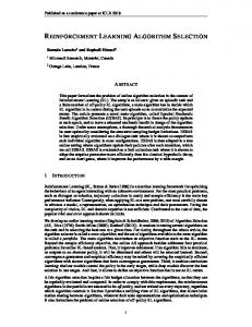
The proof is deferred to Appendix A2 . The bound consists of two terms, where the first increases with the approximation parameters (�hT , �hR ) but is independent of the dataset D, and the second has no dependence on �hT or �hR , but depends on the abstraction via nh (D), the minimal number of visits to any abstract state-action pair, and |h(S)|. The first term is small for accurate abstractions (which have small (�hT , �hR )), while the second term is small for compact abstractions (which have small |h(S)| and large nh (D)). Our goal in this paper is to select from the candidate set H an abstraction achieving the lowest loss, and we can use the bound in Theorem 1 as a proxy for that loss. (This is a common approach in existing work on abstraction selection as well as machine learning in general; see Section 5 for details.) If the size of the dataset is very small, the bound suggests that we should select a coarse abstraction to reduce estimation error. However, as the size of D grows, nh (D) increases, and the second term goes to zero while the first remains constant, implying that finer and finer abstractions will in general become preferable (see Jiang et al. (2014) for an empirical illustration). Under Assumption 1, then, the crucial question is: How much data should we require before selecting hf over hc ? If �hT and �hR were known for both abstractions, we could simply calculate an appropriate boundary from Theorem 1. However, in practice, �hT and �hR are unknown. Nevertheless, we will show that our algorithm can approximately estimate this boundary from data. In particular, we will use D to statistically test whether Q∗M hf and Q∗M hc are equal (when lifted); in general, we will reject this hypothesis after we obtain a sufficient amount of data. Perhaps surprisingly, our analysis shows that the point at which this rejection first occurs is almost the same (in the appropriate technical sense) as the point at which hf becomes preferable to hc (see Figure 1 for an illustration). Thus, we will use this hypothesis test to define a simple algorithm for abstraction selection that is near-optimal with respect to Theorem 1.
4. Proposed Algorithm and Theoretical Analysis Before proposing our algorithm, we first define the operators h BD and B h . 2 All appendices mentioned in this paper are included in an extended version available at https: //sites.google.com/a/umich.edu/nanjiang/ icml2015-abstraction.pdf.
Abstraction Selection in Model-Based RL
h
hc MD is better | MDf is better −−−−−−−−−−−−−−−−−−−−−−−−−−−−−−−−−−−−→ Null accepted by D | Null rejected by D
|D|
Figure 1. Upper part: The preferred abstraction changes as dataset size grows beyond some threshold. Lower part: Our algorithm uses the dataset to perform a hypothesis test; when dataset size exceeds some threshold, the null hypothesis will be rejected. We show that the two thresholds have bounded difference, regardless of hc and hf . h Definition 2. Given dataset D and abstraction h, BD : S×A S×A R → R is defined as follows. For any Q-value function Q ∈ RS×A , P 0 (r,s0 )∈Dh(s),a (r + γVQ (s )) h (BD Q)(s, a) = , |Dh(s),a |
where VQ (s0 ) = maxa0 ∈A Q(s0 , a0 ). We define B h as P 0 0 s0 :h(s0 )=h(s) p(s , a) · (BQ)(s , a) h P , (B Q)(s, a) = 0 s0 :h(s0 )=h(s) p(s , a) where B is the Bellman optimality operator for M , namely (BQ)(s, a) = R(s, a) + γ hP (s, a, ·), VQ (·)i. h The operator BD is a variation of the Bellman optimality h operator for MD , and B h is the same for M h . It is not hard to verify that [Q∗M h ]M and [Q∗M h ]M are, respectively, D
h fixed points of BD and B h (recall that [·]M is the lifting operation).
With these definitions, we propose Algorithm 1. It computes a particular statistic using D, and then selects hf if and only if the statistic exceeds a threshold. Algorithm 1 ComparePair(D, H, δ) assert H = {hc , hf } satisfies Assumption 1 let Q = [Q∗M hc ]M D
if
hf
BD Q − Q
∞
≥ 2 Estm(hf , D, δ/3)
(4)
then output hf , else output hc
4.1. Intuition of the Algorithm Before formally analyzing Algorithm 1, we first present an intuitive explanation for its behavior and show that it makes sensible decisions in various scenarios. The central idea is to statistically test whether [Q∗M hf ]M = [Q∗M hc ]M ,
(5)
which is equivalent (see Lemma 1 and Appendix C) to
h
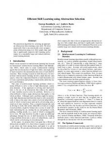
B f [Q∗ hc ]M − [Q∗ hc ]M = 0. (6) M M ∞ The LHS of Equation (6) is effectively the Bellman residual of Q∗M hc when treating M hf as the true model. Since the required quantities are not known in advance, we approximate them from data and check whether the measured error exceeds a positive rejection threshold. This gives the selection criterion of Equation (4). Consider two extreme cases. First, when M hc is a perfect homomorphism of M hf , Equation (5) always holds and we never reject the null hypothesis, thus our algorithm always returns hc . This makes sense, since the abstractions have equal approximation error but hc has lower estimation error. On the other hand, when Equation (5) does not hold, given enough data our test will reject the null hypothesis and select hf . Again, this is sensible since hf has lower approximation error, and in the limit of data the estimation error for both abstractions is zero. Of course, the usual situation is that Equation (5) does not hold but D is finite. Suppose in this case that M hf is a perfect homomorphism of M ; then Algorithm 1 can be seen as approximately comparing the bound in Theorem 1 for hf and hc , as follows. Since Appr(hf ) = 0 and the estimation errors are computable from known quantities, the only unknown quantity needed for this comparison is Appr(hc ). In principle, Appr(hc ) is a function of M and M hc , and could be approximated from data using MD and hc MD ; however, the estimate of MD will be poor when |S| is large (which is why we require abstraction in the first place). Instead, since hf is exact by assumption, we can compare M hc directly to M hf . The LHS of Equation (4) provides this estimate of Appr(hc ); see the left panel of Figure 2 for a visual illustration. In the most general scenario, where the dataset is finite and both abstractions are approximate, we need a reliable estimate of Appr(hc ) − Appr(hf ) to make the comparison using Theorem 1, but we no longer have a statistically efficient way of estimating Appr(hf ) or Appr(hc ). However, our analysis shows that even when M hf is not homomorphic to M , the three models can be seen as roughly “on the same line”, as visualized in the right panel of Figure 2. As a result, we can use the dashed line—a measure of distance between M hf and M hc —to approximate the desired difference between the solid lines. This idea is the basis for Lemma 4, which is a key ingredient in the theoretical guarantee for Algorithm 1. 4.2. Theoretical Analysis We next state the formal guarantee of our algorithm. Theorem 2. Given dataset D, if H satisfies Assumption 1, the loss of the abstraction selected by Algorithm 1 is
Abstraction Selection in Model-Based RL
Lemma 3. Let B be the Bellman optimality operator of M . For any Q : Rh(S)×A with bounded range [0, Rmax /(1−γ)], we have
B[Q]M − B h [Q]M ≤ Appr(h). ∞ Figure 2. Left panel: When M hf is a perfect homomorphism of M , we can obtain the true approximation error of M hc (solid line) by computing its approximation error w.r.t. M hf (dashed line). The two notions of approximation are equivalent, but the latter is statistically easier to estimate. Right panel: When M hf is also approximate, our theoretical analysis shows that M , M hf , and M hc are always roughly “on the same line”, so that the approximation error of M hc w.r.t. M hf (dashed line) is a good proxy for the difference between the true approximation errors of M hc and M hf (solid lines).
Lemma 4. ∀Q : RS×A with bounded range [0, Rmax /(1− γ)],
kBQ − B hc Q ∞
≤ BQ − B hf Q ∞ + B hf Q − B hc Q ∞
≤ 3 BQ − B hc Q ∞ .
bounded by
We briefly sketch the proof of Theorem 2 before proceeding to the details. Recall that our goal is to determine which abstraction has a smaller loss bound according to Theorem 1; that is, we want to check whether
n 3−γ 2 min Appr(hf ) + Estm(hf , D, δ/3), 2 (1 − γ) 1−γ o 1+γ 3−γ Appr(hc ) + Estm(hc , D, δ/3) (7) 1−γ 1−γ with probability at least 1 − δ. Equation (7) is the minimum of two terms. The first is nearly (up to a factor of O(1/(1 − γ))) the loss bound of hf using Theorem 1, and the second is nearly the loss bound of hc . Recall that Theorem 1 is our proxy for loss; therefore, the loss bound for Algorithm 1 is as good as the loss bound of the better abstraction up to a factor linear in 1/(1 − γ). Compared to Theorem 1, the estimation error terms in Equation (7) have increased from Estm(·, ·, δ) to Estm(·, ·, δ/3); however, this has little influence as Estm(·, ·, δ) depends only square-root logarithmically on 1/δ. Claim 1 (Theorem 2 is near-optimal w.r.t. Theorem 1). Equation (7) is at most the minimum of the bound in Theo1 rem 1 as applied to hf and to hc , up to a factor of O( 1−γ ). We will prove Theorem 2 with the help of the following lemmas. Their proofs are deferred to Appendices A and B. Lemma 1. For any Bellman optimality operators B1 , B2 (both operating on RS×A and having contraction rate γ), letting Q1 and Q2 be their respective fixed points, we have kQ1 − Q2 k∞ ≤
kB1 Q2 − Q2 k∞ . 1−γ
h Lemma 2. Consider BD as defined in Definition 2. For any h ∈ H and deterministic Q : RS×A with bounded range [0, Rmax /(1 − γ)], w.p. ≥ 1 − δ,
h
BD Q − B h Q ≤ Estm(h, D, δ). ∞
Appr(hc ) − Appr(hf ) ≥ Estm(hf , D, δ) − Estm(hc , D, δ), where the LHS is unknown. To approximate it, we first use Lemma 4, which implies that kB[Q∗M hc ]M − [Q∗M hc ]M k∞
≈ B[Q∗M hc ]M − B hf [Q∗M hc ]M ∞
+ B hf [Q∗M hc ]M − [Q∗M hc ]M ∞ .
(8) (9) (10)
Expression (10) is a quantity closely related to the statistic computed by our algorithm (see Equation (6)), so to establish that the statistic is a good proxy for Appr(hc ) − Appr(hf ), we will show that Appr(hc ) − Appr(hf ) ≈ Expression (8) − Expression (9). Expression (8) is easy to deal with, as the Bellman residual of [Q∗M hc ]M is a better characterization of the approximation error of hc than Appr(hc ).3 Expression (9) is a bit trickier: we know it is not an overestimate, as Lemma 3 guarantees that it is upper bounded by Appr(hf ). However, there exists the risk of underestimation: for instance, if hc aggregates all primitive states into a single abstract state, then [Q∗M hc ]M is a constant function and Expression (9) only reflects the reward error of hf , and will not change regardless of the transition error. 3
In this discussion we do not strictly distinguish between approximate homomorphism (Appr(h)) and approximate Q∗ irrelevance (the Bellman residual of Q∗M h ) in characterizing the approximation error of h. Technical details can be found in proofs and we point the readers to Li et al. (2006) for further reading.
Abstraction Selection in Model-Based RL
To deal with this, we consider two cases separately. First, when hc is the better abstraction, we have [Q∗M hc ]M ≈ Q∗M , hence
Expression (9) ≈ BQ∗M − B hf Q∗M ∞ . (11) According to Lemma 1, the RHS of Equation (11) is an alternative characterization of the approximation error of hf , so in this case we will not underestimate too much. On the other hand, when hf is better, underestimation of its approximation error only biases our selection towards the better abstraction, and is not a concern. Below we include part of the proof of Theorem 2. Proof of Theorem 2. Using Lemma 2, w.p. at least 1 − δ we have
hf ∗
BD [QM hf ]M − B hf [Q∗M hf ]M ≤ Estm(hf , D, δ/3), ∞
hc and similar concentration bounds hold for BD [Q∗M hc ]M h and BDf [Q∗M hc ]M simultaneously.
Regardless of which abstraction the algorithm selects, we can always bound its loss using Theorem 1, so it suffices to show that we can bound the loss of the selected abstraction in terms of the other. We consider each possibility in turn. If the algorithm outputs hc , we can bound the loss of hc by parameters of hf : Loss(hc , D)
2
≤
B[Q∗M hc ]M − [Q∗M hc ]M 2 D D (1 − γ) ∞
2
hf ∗ ∗ ≤
B[Q hc ]M − BD [Q hc ]M MD MD (1 − γ)2 ∞ !
h
+ BDf [Q∗M hc ]M − [Q∗M hc ]M D
≤
2 (1 − γ)2
∞
D
∞
D
2 (1 − γ)2
(13)
h
B[Q∗M hc ]M − BDf [Q∗M hc ]M
+ 2 Estm(hf , D, δ/3)
+ 2γ [Q∗M hc ]M − [Q∗M hc ]M ≤
(12)
!
∞
(14)
B[Q∗ hc ]M − B hf [Q∗ hc ]M M M ∞
+ 3 Estm(hf , D, δ/3) ! 2γ Estm(hc , D, δ/3) (15) + 1−γ � � 2 3−γ ≤ Appr(h ) + Estm(h , D, δ/3) . f f (1 − γ)2 1−γ
Equation (12) is a standard loss bound using the Bellman residual. In Equation (13), we use the triangle inequality to introduce the statistic computed by our algorithm. In the first term of Equation (14), we replace [Q∗M hc ]M by D
[Q∗M hc ]M using the fact that the Bellman operators have contraction rate γ (kBQ − BQ0 k∞ ≤ γ kQ − Q0 k∞ ), and in the second term we use the fact that the algorithm chose hc , and thus Equation (4) did not hold. Next, we apply the probabilistic guarantees stated at the beginning of the proof to remove the D subscripts on operators and Q-value functions, and finally the Appr(hf ) term appears thanks to Lemma 3. The remainder of the proof uses similar techniques and appears in Appendix B. 4.3. Extension to Arbitrary-Size Candidate Sets We briefly discuss how to extend the above algorithm and analysis to the following setting. Assumption 2. H = {h1 , . . . , h|H| }, where hi is a refinement of hi−1 for i = 2, . . . , |H|. This is the setting considered by Hallak et al. (2013), and H = {hc , hf } is the special case where |H| = 2. A natural idea is to use Algorithm 1 as a subroutine, successively comparing the best abstraction seen so far with the remaining elements in H in some order. The crucial questions are: (1) in what order should we examine the abstractions (e.g., coarse-to-fine, fine-to-coarse, or a random/adaptive order), and (2) can we adapt the analysis in Section 4.2 to show that the selected abstraction is still near-optimal w.r.t. Theorem 1 for larger H? It turns out that, if we examine abstractions in order from coarse to fine, near-optimality is preserved. Algorithm 2 provides a detailed specification for the process, and Theorem 3 gives the resulting guarantee. Algorithm 2 CompareSequence(D, H, δ) assert H = {h1 , . . . , h|H| } satisfies Assumption 2 b = h1 // start with the coarsest abstraction let h for i=2 to |H| do b = ComparePair(D, {h, b hi }, 2δ/|H|2 ) h end for b output h Theorem 3. If H satisfies Assumption 2 and has constant size, then Algorithm 2 is near-optimal w.r.t. Theorem 1, i.e., the loss of the selected abstraction is bounded w.p. at least 1 − δ by �� min Appr(h) + Estm h, D, 2δ/(3|H|2 )
h∈H
up to a factor polynomial in 1/(1 − γ).
Abstraction Selection in Model-Based RL
The biggest challenge in generalizing our analysis to the case of |H| > 2 is that the two sides of Equation (7) have different semantics—that is, the LHS is loss, while the RHS is approximation/estimation error. This means that successive comparisons cannot (naively) apply the bound transitively. Recall that, in the proof of Theorem 2, we considered the selection of hc and the selection of hf separately. It turns out that we can modify the analysis to obtain consistent, transitive semantics, but only for the case where hc is selected. This is enough for near-optimality as long as we order the abstractions from coarse to fine, avoiding the bad case of problematic abstractions. For a more detailed discussion and a proof sketch of Theorem 3, see Appendix C.
5. Related Work In this section we review prior theoretical work that is relevant to the abstraction selection problem. The discussion is summarized in Table 1. For recent empirical advances on the problem, we refer the reader to Konidaris & Barto (2009), Cobo et al. (2014), and Seijen et al. (2014). 5.1. Hypothesis Test Based Algorithms Jong & Stone (2005) (row 1) considered the factored MDP setting, where state is determined by a vector of features and an abstraction is a subset of those features. They proposed a selection procedure that statistically tests whether the optimal policy depends on certain features, aiming to aggregate states having the same optimal action and thus create a π ∗ -irrelevance abstraction. However, π ∗ -irrelevance abstractions can yield sub-optimal policies when applying Q-learning even with infinite data, so this method is not statistically consistent (Li et al., 2006, Theorem 4). Hallak et al. (2013) (row 2), in the work most closely related to ours, considered the setting of Assumption 2 and suggested comparing hc and hf by statistically testing whether M hc is a perfect homomorphism of M hf using D. They showed theoretically that their procedure will asymptotically identify any abstraction that is a perfect homomorphism of M . However, if all the candidate abstractions are approximate, or the dataset is finite, their analysis does not apply. Nevertheless, there are interesting similarities between our Algorithm 1 and the method of Hallak et al. (2013): both algorithms test relative properties of hc and hf so as to avoid the large primitive representation, and both choose the coarser abstraction unless a statistical test rejects the null hypothesis that hc and hf are (in some sense) equivalent. However, our analysis shows that this type of algorithm can still have provable guarantees even when the data are insufficient and the abstractions are approximate—in fact, it can be near-optimal with respect to a loss bound. There are several important technical differences between
our algorithm and that of Hallak et al. (2013): (1) We use Q∗ -irrelevance as the equivalence criterion in our hypothesis test, whereas they use homomorphism; Q∗ -irrelevance is a strictly more general relationship than homomorphism (Li et al., 2006, Theorem 2) that avoids the problematic L1 norm as a characterization of estimation error (Maillard et al., 2014) and enables convenient mathematical tools for h finite sample analysis (e.g., the BD operator). (2) We fully specify the rejection threshold for the hypothesis test (up to the probability guarantee δ) without introducing additional hyperparameters, while in their work the rate of threshold decay as the dataset grows is left to the practitioner. This choice can have a significant impact on the transient behavior of the algorithm. 5.2. Reduction to Offline Policy Evaluation Inspired by model selection techniques in supervised learning, abstractions can also be selected using a crossvalidation procedure: if a second dataset D0 is given independently of D, then we can evaluate the policies computed ∗ under different abstractions from D (i.e., {πM h : h ∈ H}) D 0 on D . This turns the abstraction selection problem into an offline policy evaluation problem, and the loss guarantee depends entirely on the accuracy of the offline evaluation estimator. Below we briefly discuss two commonly used estimators; see more details in Paduraru (2013). 5.2.1. I MPORTANCE S AMPLING E STIMATOR When D0 comprises trajectories sampled according to a known stochastic policy, importance sampling (row 3) can be used to obtain an unbiased estimate of the value, with respect to the initial state distribution in the data, of the policy under evaluation (Precup et al., 2000). The variance of this estimate has no dependence on the size of the primitive state space, but in general has exponential dependence on the horizon (Mandel et al., 2014): to evaluate a deterministic policy π, the estimator must restrict itself to trajectories in which the action choice at each time step exactly agrees with π. If, for instance, the sampled trajectories are L = 1/(1 − γ) steps long and generated by choosing uniformly random actions, then the probability of any single trajectory being useful is 1/|A|L , hence the proportion of data available for estimation decreases exponentially with L. Even so, importance sampling can be practical and has been successfully applied to real-world problems with very short horizons (Li et al., 2011; Mandel et al., 2014). 5.2.2. M ODEL -BASED E STIMATOR For problems with longer horizons, an alternative is the model-based estimator (row 4), which uses D0 to construct a model MD0 (without abstraction) and then evaluates a π policy π by computing VM . However, this approach is not D0
Abstraction Selection in Model-Based RL Table 1. Comparison of algorithms that can be applied to the abstraction selection problem. If an entry exhibits a desired property (which we judge by generality and practicality), we mark it as bold. In the first row we provide the properties of model-based RL with primitive representation as a baseline to compare against.
No Abstraction 1.Jong & Stone (2005)
Finite Sample Guarantee Dependence on Dependence Representation on Horizon |S| Polynomial [No guarantee]
2.Hallak et al. (2013)
[Only asymptotic guarantee]
3.Importance Sampling 4.Model-based Estimator 5.Farahmand & Szepesv´ari (2011) Our method
No |S| Size of regressor abstraction Size of best abstraction
Assumption on Candidate Abstractions Subsets of state features Successive refinements
Exponential Polynomial Polynomial
No No No
Polynomial
Successive refinements
Tuning Hyperparameters
Optimization Objective
Noa
-
Statistical test threshold as a function of sample size No No Choice of regressor abstraction No
Coarseness of perfect homomorphisms Loss Loss Bellman residual loss bound Approximate homomorphism loss bound
a
Their algorithm has a single parameter which is the p-value threshold for hypothesis test, and they suggest using 0.05 in practice. In fact, all the methods listed in this table except the first 3 rows require a similar confidence level parameter.
useful in our setting, since MD0 is itself hard to estimate:
π π − VM the bound on the estimation error VM
depends D0 ∞ on the minimal state visitation number, and therefore on |S| (Mannor et al., 2007; Paduraru et al., 2008). Alternatively, the validation model can be estimated under an abstraction to avoid the dependence on |S|, but this solution is circular: if we knew a good abstraction for policy evaluation, we could have used it to obtain a good policy in the first place. For instance, Farahmand & Szepesv´ari (2011) (row 5) proposed an offline policy evaluation procedure that selects value functions (from which policies are computed) based on their estimated Bellman residuals, which are estimated with the help of an additional regressor that learns BQ from data for the candidate Qs. The theoretical guarantee for this method depends on the accuracy of the regressor (see their Theorem 2, especially the dependence on ¯bk ). For the reason noted above, this is problematic in our setting: h the abstractions are themselves regressors (where BD Q is the function being learned), so if we knew how to select a good abstraction for regression, then the same one could have been used to learn a policy instead. 5.3. The Online Setting Ortner et al. (2014) proposed a representation (abstraction) selection algorithm in the online exploration and exploitation setting that tests whether a representation faithfully predicts the return of a roll-out trajectory. Their regret bound depends on the sum of sizes of the state spaces for all repre-
sentations under consideration (see their Theorem 3). While the online setting has additional complications, in our offline setting this bound is loose and can be improved simply by selecting the finest available abstraction. On the other hand, although our algorithm assumes structure in the candidate abstractions (they must be successive refinements), our loss bound depends only on the best abstraction.
6. Conclusion In this paper we considered the abstraction selection problem in the setting where the amount of data is limited and candidate abstractions may all be approximate. As far as we know, there is no provable algorithm that achieves significantly better dependence on representation (than the baseline of the primitive state space) without blowing up the dependence on horizon exponentially, suggesting that the problem is generally hard. Our work showed that, when the candidate abstractions satisfy certain refinement assumptions, a simple hypothesis test based algorithm can select abstractions with a loss bound only depending on the best abstraction up to a factor polynomial in horizon. The theoretical analysis is fundamentally based on the approximation/estimation error trade-off with finite data, departing from the asymptotic analysis of previous work that only considered perfect abstractions in the limit of data. Possible directions for future work include relaxing the assumption (e.g., to the setting of feature selection), and developing heuristic algorithms based on the algorithmic ideas provided in this paper.
Abstraction Selection in Model-Based RL
Acknowledgement This work was supported by NSF grant IIS-1319365. Any opinions, findings, conclusions, or recommendations expressed here are those of the authors and do not necessarily reflect the views of the sponsors.
References Cobo, Luis C, Subramanian, Kaushik, Isbell, Charles L, Lanterman, Aaron D, and Thomaz, Andrea L. Abstraction from demonstration for efficient reinforcement learning in high-dimensional domains. Artificial Intelligence, 216: 103–128, 2014. Dinculescu, Monica and Precup, Doina. Approximate predictive representations of partially observable systems. In Proceedings of the 27th International Conference on Machine Learning (ICML-10), pp. 895–902, 2010. Even-Dar, Eyal and Mansour, Yishay. Approximate equivalence of Markov decision processes. In Learning Theory and Kernel Machines, pp. 581–594. 2003. Farahmand, Amir-massoud and Szepesv´ari, Csaba. Model selection in reinforcement learning. Machine learning, 85(3):299–332, 2011. Hallak, Assaf, Di-Castro, Dotan, and Mannor, Shie. Model selection in markovian processes. In Proceedings of the 19th ACM SIGKDD Conference on Knowledge Discovery and Data mining, pp. 374–382, 2013. Jiang, Nan, Singh, Satinder, and Lewis, Richard. Improving UCT planning via approximate homomorphisms. In Proceedings of the 13th International Conference on Autonomous Agents and Multi-Agent Systems, pp. 1289– 1296, 2014. Jong, Nicholas K and Stone, Peter. State abstraction discovery from irrelevant state variables. In Proceedings of the 19th International Joint Conference on Artificial Intelligence, pp. 752–757, 2005. Konidaris, George and Barto, Andrew. Efficient Skill Learning using Abstraction Selection. In Proceedings of the 21st International Joint Conference on Artificial Intelligence, 2009. Lever, Guy, Baldassarre, Luca, Gretton, Arthur, Pontil, Massimiliano, and Gr¨unew¨alder, Steffen. Modelling transition dynamics in MDPs with RKHS embeddings. In Proceedings of the 29th International Conference on Machine Learning (ICML-12), pp. 535–542, 2012. Li, Lihong, Walsh, Thomas J, and Littman, Michael L. Towards a unified theory of state abstraction for MDPs. In Proceedings of the 9th International Symposium on Artificial Intelligence and Mathematics, pp. 531–539, 2006.
Li, Lihong, Chu, Wei, Langford, John, and Wang, Xuanhui. Unbiased offline evaluation of contextual-bandit-based news article recommendation algorithms. In Proceedings of the 4th ACM International Conference on Web Search and Data Mining, pp. 297–306, 2011. Maillard, Odalric-Ambrym, Mann, Timothy A, and Mannor, Shie. ”How hard is my MDP?” The distribution-norm to the rescue. In Advances in Neural Information Processing Systems, pp. 1835–1843, 2014. Mandel, Travis, Liu, Yun-En, Levine, Sergey, Brunskill, Emma, and Popovic, Zoran. Offline policy evaluation across representations with applications to educational games. In Proceedings of the 13th International Conference on Autonomous Agents and Multi-Agent Systems, pp. 1077–1084, 2014. Mannor, Shie, Simester, Duncan, Sun, Peng, and Tsitsiklis, John N. Bias and variance approximation in value function estimates. Management Science, 53(2):308–322, 2007. ´ Ormoneit, Dirk and Sen, Saunak. Kernel-based reinforcement learning. Machine learning, 49(2-3):161–178, 2002. Ortner, Ronald, Maillard, Odalric-Ambrym, and Ryabko, Daniil. Selecting Near-Optimal Approximate State Representations in Reinforcement Learning. arXiv preprint arXiv:1405.2652, 2014. Paduraru, Cosmin. Off-policy Evaluation in Markov Decision Processes. PhD thesis, McGill University, 2013. Paduraru, Cosmin, Kaplow, Robert, Precup, Doina, and Pineau, Joelle. Model-based reinforcement learning with state aggregation. In 8th European Workshop on Reinforcement Learning, 2008. Parr, Ronald, Li, Lihong, Taylor, Gavin, Painter-Wakefield, Christopher, and Littman, Michael L. An analysis of linear models, linear value-function approximation, and feature selection for reinforcement learning. In Proceedings of the 25th International Conference on Machine Learning, pp. 752–759, 2008. Precup, Doina, Sutton, Richard S, and Singh, Satinder. Eligibility traces for off-policy policy evaluation. In Proceedings of the 17th International Conference on Machine Learning, pp. 759–766, 2000. Ravindran, Balaraman. An algebraic approach to abstraction in reinforcement learning. PhD thesis, University of Massachusetts Amherst, 2004.
Abstraction Selection in Model-Based RL
Ravindran, Balaraman and Barto, Andrew. Approximate homomorphisms: A framework for nonexact minimization in Markov decision processes. In Proceedings of the 5th International Conference on Knowledge-Based Computer Systems, 2004. Seijen, Harm, Whiteson, Shimon, and Kester, Leon. Efficient abstraction selection in reinforcement learning. Computational Intelligence, 30(4):657–699, 2014. Singh, Satinder and Yee, Richard. An upper bound on the loss from approximate optimal-value functions. Machine Learning, 16(3):227–233, 1994. Sutton, Richard and Barto, Andrew. Introduction to reinforcement learning. MIT Press, 1998. Sutton, Richard S, McAllester, David A, Singh, Satinder P, and Mansour, Yishay. Policy gradient methods for reinforcement learning with function approximation. In Advances in Neural Information Processing Systems, volume 99, pp. 1057–1063, 1999. Talvitie, Erik and Singh, Satinder. Learning to make predictions in partially observable environments without a generative model. Journal of Artificial Intelligence Research (JAIR), 42:353–392, 2011.
Abstraction Selection in Model-Based RL
A. Proof of Theorem 1
D = R(s, a) + γ
kQ1 − Q2 k∞
P (s, a, s0 ), VQ (·) −
s0 ∈h−1 (·)
We first prove Lemma 1, 2 and 3. Proof of Lemma 1. ∀s ∈ S, a ∈ A,
X
Rmax E 2(1 − γ)
D Rmax E − Rh (h(s), a) − γ P h (h(s), a, ·), VQ (·) − 2(1 − γ) Rmax ≤ �hR + �hT = Appr(h). 2(1 − γ)
= kB1 Q1 − B1 Q2 + B1 Q2 − Q2 k∞ ≤ γ kQ1 − Q2 k∞ + kB1 Q2 − Q2 k∞ . Hence the bound follows. Note that this result subsumes the standard Bellman residual bound, when we let Q2 be an approximate Q-value function (e.g. [Q∗M h ]M , where B2 = B h ), and Q1 be the true optimal value function Q∗M (where B1 = B). Furthermore, thanks to the definition of B h , we can form, namely bounding
∗use this∗bound in an alternative
Q − [Q h ]M by Q∗ − B h Q∗ . We will use M M M ∞ M ∞ both forms (and sometimes treating M h as the true model) throughout the theoretical analysis depending on the context.
Proof of Lemma 2. According to Definition 2, h (BD Q)(s, a) is the average of r + γVQ (s0 ) for (r, s0 ) ∈ Dh(s),a , which are independent random variables with bounded range [0, Rmax /(1 − γ)]. When |Dh(s),a | > 0,4 it is straight-forward to �verify that for any deterministic h Q, (B h Q)(s, a) = ED (BD Q)(s, a) |Dh(s),a | > 0 . Hence, Hoeffding’s inquality applies, ∀t > 0, n o h PD (BD Q)(s, a) − (B h Q)(s, a) ≥ t � � 2t2 |Dx,a | ≤ 2 exp − 2 . Rmax /(1 − γ)2 Now we find t that makes the inequality hold for all (s, a) ∈ S × A simultaneously w.p. at least 1 − δ via union h bound. Note, however, that BD Q (and B h Q) takes constant value among states aggregated by h, hence we only have |h(S)||A| events in the union bound instead of |S||A| ones. The t that satisfies our requirement turns out to be s Rmax 1 2|h(S)||A| t= log = Estm(h, D, δ), h 1 − γ 2n (D) δ and this completes the proof.
This completes the proof. Proof of Theorem 1. Let [Q∗M h ]M denote Q∗M h lifted to D D M , namely [Q∗M h ]M (s) = Q∗M h (h(s)). We have, D
D
π∗ h
∗
VM − V MD M
∞
2 ≤ 1−γ 2 ≤ 1−γ 2 = 1−γ
∗
QM − [Q∗M h ]M (Singh & Yee, 1994) D ∞
� �
kQ∗M − [Q∗M h ]M k∞ + [Q∗M h ]M − [Q∗M h ]M D ∞
� �
kQ∗M − [Q∗M h ]M k∞ + Q∗M h − Q∗M h . D
∞
According to Lemma 3, the first term in the bracket can be bounded as:
B[Q∗ h ]M − B h [Q∗ h ]M M M ∗ ∗ ∞ kQM − [QM h ]M k∞ ≤ 1−γ Appr(h) . ≤ 1−γ For the second term, we use Lemma 1 by letting B1 = B hf h and B2 = BDf , and then apply Lemma 2: w.p. at least 1 − δ,
∗
QM h − Q∗M h D
∞
h ∗
B [Q h ]M − B h [Q∗ h ]M D M M ∞ ≤ 1−γ Estm(h, D, δ) ≤ . 1−γ
Combining the bounds for the two terms and the theorem follows.
B. Proof of Theorem 2 We first prove the remaining Lemma.
Proof of Lemma 3. ∀s ∈ S, a ∈ A, (B[Q]M )(s, a) − (B h [Q]M )(s, a) D E = R(s, a) + γ P (s, a, ·), [VQ ]M (·) D E − Rh (h(s), a) − γ P h (h(s), a, ·), VQ (·) 4 When |Dh(s),a | = 0, nh (D) = 0 and the RHS of the bound goes to infinity, which promises nothing and is always correct.
Proof of Lemma 4. The left inequality is trivial from the triangular inequality. To
prove the right inequality,
BQ − B hf Q and B hf Q − B hc Q by we bound ∞ ∞
BQ − B hc Q separately. The key is to notice that, for ∞ any x ∈ hf (S), (B hf Q)(x, a) is always a convex average of {(BQ)(s, a) : s ∈ h−1 f (x)}.
Abstraction Selection in Model-Based RL
We first show BQ − B hf Q ∞ ≤ 2 BQ − B hc Q ∞ . Notice that there exist s, s0 ∈ S, a ∈ A s.t. hf (s) = hf (s0 ) and
|(BQ)(s, a) − (BQ)(s0 , a)| ≥ BQ − B hf Q ∞ .
! + Estm(hf , D, δ/3) ≤
≥
max
|(BQ)(s, a) − (BQ)(s0 , a)| / 2
max
|(BQ)(s, a) − (BQ)(s0 , a)| / 2
hc (s)=hc (s0 ) a∈A
hf (s)=hf (s0 ) a∈A
hf
≥ BQ − B
h
B f [Q∗ hc ]M − B[Q∗ hc ]M M M ∞ !
Using the same argument on hc , it is obvious that
BQ − B hc Q ∞ ≥
2 (1 − γ)2
(16)
+ 2γ kQ∗M − [Q∗M hc ]M k∞ + Estm(hf , D, δ/3) ≤
Q ∞ / 2,
hence the bound follows.
Next we show B hf Q − B hc Q ∞ ≤ BQ − B hc Q ∞ . Consider the state-action pair that achieves the max norm
of B hf Q − B hc Q ∞ , i.e.
+ Estm(hf , D, δ/3) ≤
. ∞
will be no less than h (B f Q)(s, a) − (B hc Q)(s, a) , which implies that
h
B f Q − B hc Q ≤ BQ − B hc Q . ∞ ∞
3−γ kB[Q∗M hc ]M − [Q∗M hc ]M k∞ 1−γ
∞
≤
≤
! + 2 Estm(hf , D, δ/3)
3−γ 2 kB[Q∗M hc ]M − [Q∗M hc ]M k∞ (1 − γ)2 1 − γ
h
− BDf [Q∗M hc ]M − [Q∗M hc ]M + 2 Estm(hf , D, δ/3) D D ∞ !
∗
+ (1 + γ) [QM hc ]M − [Q∗M hc ]M D
or (BQ)(s00 , a) − (B hc Q)(s00 , a)
2 (1 − γ)2
h
− BDf [Q∗M hc ]M − [Q∗M hc ]M
h
(B f Q)(s, a) − (B hc Q)(s, a) = B hf Q − B hc Q
Since (B hf Q)(s, a) is a convex average of {(BQ)(s0 , a) : hf (s0 ) = hf (s)}, there always exists s0 : hf (s0 ) = hf (s) such that (BQ)(s0 , a) ≥ (B hf Q)(s, a), and s00 : hf (s00 ) = hf (s) such that (BQ)(s00 , a) ≤ (B hf Q)(s, a). Note that (B hc Q)(s, a) = (B hc Q)(s0 , a) = (B hc Q)(s00 , a), hence either (BQ)(s0 , a) − (B hc Q)(s0 , a)
2 3 B hc [Q∗M hc ]M − B[Q∗M hc ]M ∞ 2 (1 − γ)
− B hf [Q∗M hc ]M − B hc [Q∗M hc ]M ∞ 2γ + kB[Q∗M hc ]M − [Q∗M hc ]M k∞ 1−γ !
2 (1 − γ)2 +
∞
3−γ
B[Q∗ hc ]M − B hc [Q∗ hc ]M M M ∞ 1−γ !
1+γ Estm(hc , D, δ/3) 1−γ
2 = (1 − γ)2
(17)
! 3−γ 1+γ Appr(hc ) + Estm(hc , D, δ/3) . 1−γ 1−γ
This completes the proof. Proof of Theorem 2 (continued). Similarly, if the algorithm outputs hf , Loss(hf , D)
2
∗
≤
QM − [Q∗M hf ]M 1−γ ∞
!
∗
∗
+
[QM hf ]M − [Q hf ]M MD
≤
2 (1 − γ)2
The derivation is similar to the previous one, with a few small changes. In Equation (16), instead of the Bellman residual we use Lemma 1 to bound the value difference. We also replace Q∗M with [Q∗M hc ]M , and use Lemma 4 to introduce a term similar to the statistic computed by the algorithm. Then, using the probabilistic guarantees stated at the beginning, we obtain exactly that statistic, and bound it using Equation (4). Finally, Appr(hc ) appears from Lemma 3 and Estm(hc ) from the probabilistic guarantees.
∞
C. Proof Sketch of Theorem 3
h ∗
B f QM − BQ∗M ∞
We first prove a lemma on Bellman residuals.
Abstraction Selection in Model-Based RL
Lemma 5. For any Q-value function Q : RS×A , kBQ − Qk∞ ≤ (1 + γ) kQ − Q∗M k∞ .
Proof.
� 2
hc ∗ ∗
B[Q hc ]M − BD [QM hc ]M M (1 − γ)2 ∞ � + 2 Estm(hc , D, δ 0 )
� 2
hc ∗ ∗ ≤
B[Q hc ]M − BD [Q hc ]M MD MD (1 − γ)2 ∞
�
∗ + 2γ [QM hc ]M − [Q∗M hc ]M + 2 Estm(hc , D, δ 0 ) ,
≤
D
kBQ − Qk∞ = kBQ − Q∗M + Q∗M − Qk∞ ≤ kBQ − BQ∗M k∞ + kQ∗M − Qk∞ ≤ γ kQ∗M − Qk∞ + kQ∗M − Qk∞ = (1 + γ) kQ∗M − Qk∞ . So the lemma follows. Theorem 3 will a direct corollary of Lemma 6, by noticing that the loss of the selected abstraction can be upper bounded by the LHS of Equation (18). Lemma 6. Suppose Assumption 2 holds. Let hbi be the bestso-far abstraction among h1 , . . . , hi found by Algorithm 2, then for δ 0 = 2δ/(3|H|2 ), the following bound holds w.p. ≥ 1 − δ: ∀i = 1, 2, . . . , |H|,
∗
[QM hci ]M − Q∗M
∞
+
1 Estm(hbi , D, δ 0 ) 1−γ
1 � ≤ poly · min (Appr(h) + Estm(h, D, δ 0 )) . 1 − γ h∈{h1 ,...,hi } (18)
Proof Sketch. For every pair of possible comparison we require the 3 probabilistic guarantees in the proof of Theorem 2 to hold, hence by union bound we can guarantee that each of them occurs w.p. at least 1 − δ 0 . Then, we prove the lemma by induction. For the case of i = 1, it holds obviously from Theorem 1, by noticing that the LHS of Lemma 6 is an intermediate step of proving Theorem 1 (up to 2/(1 − γ)), and the RHS is consistent with the final bound. Suppose the induction assumption holds for i, and consider the comparison between hc = hbi and
hf = hi+1 . If hc is selected, we only need to prove that [Q∗M hc ]M − Q∗M ∞ + 1 0 1−γ Estm(hc , D, δ ) can be bounded by Appr(hf ) and 0 Estm(hf , D, δ ), which is possible by slightly adapting the previous analysis. In particular, � � 2 1 k[Q∗M hc ]M − Q∗M k∞ + Estm(hc , D, δ 0 ) 1−γ 1−γ �
2
B[Q∗ hc ]M − B hc [Q∗ hc ]M ≤ M M ∞ (1 − γ)2 � + Estm(hc , D, δ 0 )
∞
and now we arrive at Equation (12), up to some extra dependence on Estm(hc , D, δ 0 ) (which we can always afford), and the difference between δ and δ 0 . Following the rest part of the previous analysis we will have the desired bound. If hf is selected, the beginning part of the previous analysis can be adapted much more easily: � �
1 2
∗ ∗ 0 + ] − Q Estm(h , D, δ )
[[QM hf M f M 1−γ 1−γ ∞ � �
2
BQ∗M − B hf Q∗M + Estm(hf , D, δ 0 ) , ≤ ∞ (1 − γ)2 and now we are at Equation (16). This time, however, we cannot follow the previous analysis all the way to the end, as our induction assumption promises nothing for Appr(hc ) and Estm(hc ). Instead, we can departure from Equation (17): (17) ≤
2 (1 − γ)2 +
(3 − γ)(1 + γ) k[Q∗M hc ]M − Q∗M k∞ 1−γ !
1+γ Estm(hc , D, δ 0 ) , 1−γ
which follows from Lemma 5. Now we can apply our induction assumption, and this shows that the induction assumption holds for i + 1, so the lemma follows.