Accelerating Fluid Registration Algorithm on Multi-FPGA Platforms

Accelerating Fluid Registration Algorithm on Multi-FPGA Platforms Jason Cong, Muhuan Huang and Yi Zou Computer Science Department University of California, Los Angeles Los Angeles, CA 90095, USA

Abstract—In the clinical applications, medical image registrations on the images taken from different times and/or through different modalities are needed in order to have an objective clinical assessment of the patient. Viscous fluid registration is a powerful PDE-based method that can register large deformations in the imaging process. This paper presents our implementation of the fluid registration algorithm on a multi-FPGA platform Convey HC-1. We obtain a 35X speedup versus single-threaded software on a CPU. The implementation is achieved using a high-level synthesis (HLS) tool, with additional source-code level optimizations including fixedpoint conversion, tiling, prefetching, data-reuse, and streaming across modules using a ghost zone (time-tiling) approach. The experience of this case study also identifies further automation steps needed by existing HLS software.

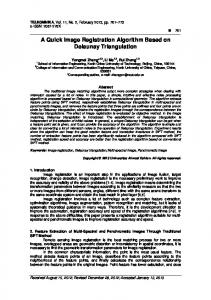
I. I NTRODUCTION Image registration tries to find a transformation function of the coordinate system of one image into the coordinate system of another image. The ultimate goal is to better align the two images. In the clinical setting, we may want to perform image registration of the image studies taken of the same patient to see the progressive development of the illness (e.g., tumors). Image registration is also used for remote sensing and computer vision as well. While there are various kinds of image registration algorithms, we can normally break the algorithm into four parts: transform, interpolator, metric, and the optimizer on the metric. Fig. 1 shows the block diagram of a typical image registration algorithm. Transform declares the type of transforms (or coordinate mapping) from the coordinates in the reference image to the coordinates in the target image space. An affine transform models translation, scaling, rotation, shear mapping, etc. A rigid transform model is a subset of the affine transform which only allows translation, rotation and reflection. The deformable transform allows a more general transform formulation which can map a coordinate in the reference image space into any coordinate in the target image space. Interpolator performs interpolation in order to obtain the pixel value at the non-integer coordinates. Metric is the objective we need to optimize. Typical similarity metrics for the two images include the sum of squared differences (SSD), mutual information and cross-correlation etc. In order to restrict the transform or displacement functions, an additional regularization term on the transform or the

Registration Method Target Image

Metric

Optimizer

Interpolator Reference Image

Transform

Figure 1: Block Diagram of Image Registration Algorithms displacement is also needed. Typical optimization schemes include steepest decent, conjugate gradient and some global optimization algorithms. Pioneer work on FPGA-based medical image registration includes FAIR [1], FAIR II [2] and the recent work by the same group that uses the sub-volume mutual information based method [3]. FAIR and FAIR II all use mutual information as the optimization metric. Mutual information (MI) is particularly useful for multi-modality (e.g., CT vs MRI) registration. Rigid transform is used in FAIR and FAIR II. Rigid transform can be used to find the global alignments, but most distortions (such as respiration effects) in the imaging process requires a deformable transform. The sub-volume MI based method [3] hierarchically divides the image studies into sub-volumes, and allows rigid transform to be applied on each sub-volume. Clearly, this is a deformable transform because different sub-volumes may use different rigid transforms. The drawback is that the transform is not smooth—in particular for the voxels at the boundaries of a sub-volume. In this work we try to accelerate a PDE-based nonparametric registration called fluid registration. Fluid registration regularizes the deformation using a fluid PDE equation, and it allows registrations of large deformations. Fluid regularizers ensure that the transform function is smooth. Currently, the speed of the algorithm cannot meet the clinical need. It may take close to one hour to finish up a typical registration (image with size 2563 , 500 iterations) on a standard workstation. The application is both computeintensive and data-intensive. This work tries to accelerate the fluid registration algorithm on a multi-FPGA platform. The highlights of our implementation are listed below. First, in the fluid registration algorithm that we implement, the transform is described through a point-wise displacement

S

interp T

interpT

updateF

u

updateU

f

v

updateV

Figure 3: Dataflow Between Procedures Figure 2: System Diagram of Convey HC-1 Hybrid Computer function u1 , u2 , u3 where a point at (i, j, k) will get mapped to coordinate ((i − u1 (i, j, k), j − u2 (i, j, k), k − u3 (i, j, k)); thus, each voxel (rather than a sub-volume) can move independently in a deformable fashion. Second, to accelerate this dataintensive application, we employ several source-code level optimizations that include fixed-point conversion, tiling, prefetching, data-reuse, and streaming across modules using a ghost zone (time-tiling) approach. We evaluate the impact of these optimizations. Third, we use a high-level synthesis tool to speed up the implementation process, and identify their pros and cons through this complex case study. We have reference code that uses either sum of square differences (SSD) or mutual information as the optimization metric. Currently, we apply the registration on the image studies with the same modality; thus, we use simpler SSD as the optimization metric. II. F LUID R EGISTRATION A LGORITHM R EVIEW Fluid registration [4] performs smoothing on the velocity field v (or so-called incremental deformation field) rather than the total deformation field u. Solving large-scale PDE, especially for 3D image registration, (e.g., Navier-Stokes PDE for fluid registration), is a computationally expensive process. Bro-Nielsen et al. [5] proposed to use a scale-space convolution filter to accelerate the smoothing process. Our baseline implementation is a variant of the implementation in [5], except that we simply use a Gaussian filter to smooth the velocity field. Gaussian filter is used in the optical-flow based Demons algorithm [6], and also used in several more recent fluid registration work [7], [8] as well. The key mathematical derivations for fluid registration can be seen in [4], [5], [9]. Here we briefly review them for completeness. The two image studies are S and T . The deformation field is termed u. In each iteration, we first perform linear interpolation based on the deformation field: Te(x, t) = T (x − u(x, t))

(1)

We obtain the force field using the derivative of an L2 SSD

metric: f (x, u(x, t)) = −[Te(x, t) − S(x)]∇Te(x, t)

(2)

Instantaneous velocity v(x, t) can be obtained by solving the fluid PDE: µ∆v(x, t) + (µ + λ)∇div v(x, t) = f (x, u(x, t))

(3)

In our implementation, we simply use a Gaussian convolution as in [7], [8]. v(x, t) ≈ Gσ ∗ f (x, u(x, t))

(4)

We use the recursive Gaussian infinite impulse response (IIR) filter proposed by Alvarez and Mazorra [10]. This IIR only needs two MADD operation per dimension. This is the fastest 3D Gaussian filter we know of. It is one magnitude faster than the FFT-based convolution used in [8], and should also be faster than direct convolution and other recursive Gaussian IIR e.g., those by Young [11]. Note an additional normalization step can be fused into the subsequent computation procedures. After that we obtain an updated deformation field by solving the PDE du(x, t)/dt = v(x, t) − v(x, t)∇u(x, t), using an explicit Euler scheme: R(x, ti ) = (v(x, ti ) − v(x, ti )∇u(x, ti )) u(x, t

i+1

i

) = u(x, t ) + (t

i+1

− t )R(x, t ) i

i

(5) (6)

The advancement of timestep needs to be bounded so that (ti+1 − ti ) max∥R(x, ti )∥2 does not exceed the maximum displacement allowed in one iteration. III. C ONVEY HC-1 M ULTI -FPGA P LATFORM We use the Convey HC-1 [12] as the experimental platform for this implementation. The multi-FPGA platform Convey HC-1 uses an interleaved memory scheme. Memory requests are allowed for 8-bit,16-bit, 32-bit or 64-bit accesses only. Different FPGAs access the off-chip memory using a shared memory model. The system employs an onboard crossbar to realize the interconnection. Figure 2 shows the system diagram for the Convey HC-1. The HC-1 platform has four user FPGAs (Virtex 5 LX330). Each FPGA is presented with 16 external memory access ports. (Eight physical memory ports are connected to eight memory controllers which run at 300MHZ. Core design runs at 150MHZ. Thus, effectively the design on each

Mem requests for read

/ / I n p u t : a r r a y u tmp / / O u t p u t : a r r a y u tmp a f t e r i n−p l a c e u p d a t e / / Backward : u [ 0 ] = u [ 0 ] ∗ c1 ; f o r ( i = 1 ; i < N−1; i ++) u [ i ] = u [ i ] + u [ i −1] ∗ c2 ; / / Forward : u [N−1] = u [N−1] ∗ c1 ; f o r ( i = N−2; i >= 0 ; i −−) u [ i ] = u [ i ] + u [ i + 1 ] ∗ c2 ;

Address Generator

Forward Mem responses processing for read unit

gn op -g in P

re ff ub

Backward Mem requests processing for write unit

Figure 4: 1D IIR PE

Figure 5: 1D Gaussian IIR

FPGA is presented with 16 “logical” memory access ports through time multiplexing.) Our application is data intensive and needs to read and write a lot of data. The ratio between computation and the data accesses is fairly low. Because the size of the 3D images are too big to fit in the on-chip RAM, we need to use off-chip DRAM extensively. Convey HC-1 provides a large bandwidth (claimed to have 80GB/s peak bandwidth) for coprocessor side memory. We did spend significant effort on the selection of a good heterogenous platform that fits our needs. Before deciding on the Convey HC-1 platform, we also evaluated several alternatives. Xilinx XUPV5 board [13] has only one DIMM and the off-chip memory bandwidth is less than 1GB/s. In the Nallatech FSB Development System [14], the FPGA coprocessor accesses the system memory through front-side bus and the bandwidth is limited to the bandwidth of FSB (around 8GB/s).

Gaussian IIR because the σ used in our reference implementation is relatively large. Recursive IIR smoothing works through the sweeping of the 3D image in the three dimensions (or six directions) sequentially. Suppose the image size is 2563 , we need to perform 2562 1D IIRs in each dimension. Our 1D IIR uses the recursive computation in each direction:

IV. M ODULE - LEVEL I MPLEMENTATION The whole fluid registration in our baseline contains the following computation kernels: interp which corresponds to Eq. 1; updateF which corresponds to Eq. 2; updateV which corresponds to Eq. 4 and updateU which corresponds to Eq. 5 and 6. The registration algorithm is an iterative process that repeatedly calls these procedures. The dataflow between the procedures is shown in Fig. 3. When non-core parts (File IO etc.) are excluded, it takes around 6s per iteration on a Intel Xeon 2.0GHZ CPU. Approximately 45% of the time is spent on Gaussian smoothing, and 35% on displacement update, 15% on interpolation, and 5% on force calculation. A. Gaussian Smoothing Gaussian smoothing essentially performs e = Gσ ⊗ A A

(7)

where Gσ is a Gaussian function and ⊗ is the convolution operator. The 3D Gaussian function is Gσ (x, y, z) =

1 (2πσ 2 )

3 2

e−

x2 +y 2 +z 2 2σ 2

(8)

There are many algorithms and implementations of Gaussian smoothing: FFT-based convolution, direct convolution, and recursive impulse infinite response (IIR) filtering. We use

y(n) ≈ a ∗ x(n) + b ∗ y(n − 1)

(9)

where y(n) denotes the new signal sequence that is generated by the IIR, and x(n) means the input signal sequence. Fig. 5 shows the code for 1D IIR. We design the hardware for the Gaussian IIR in a way that there is a large number of parallel PEs that talk to different memory ports. Each processing element (PE) is a hardware unit that can compute a group of 1D IIR in an interleaved fashion. (We need to do such interleaving to hide the latency of the MADD unit.) Each PE is composed of three components. One component is the address generator hardware unit that keeps sending memory access requests into one memory access port. In parallel with the address generator, the main task-level pipeline includes the backward processing unit and forward processing unit. The backward processing unit reads memory responses, performs computation, and writes data into the on-chip BRAM (ping-pong buffer). The forward processing unit reads data from the ping-pong buffer and sends requests to another memory access port. The backward processing unit and the forward processing unit work in parallel. The computation within the forward processing unit and backward processing unit are deeply pipelined using standard loop pipelining techniques. We realize eight PEs on each FPGA. Our multi-FPGA design incorporates 32 PEs and utilizes all the memory access ports available in the platform. Additional implementation issues of this module on multi-core CPU, many-core GPU, and FPGAs is shown in [15]. B. Displacement Update This is a kernel that mainly performs stencil data access and performs some finite difference calculation. The input of this module is the deformation field u and velocity field v, the output of this module is the updated deformation field.

Memory requests for read Address generator for v

Memory responses for read

Address generator for u

u

Reuse buffer

Compute unit

Memory requests for write

Address generator for T

uTo interpolation module

Figure 6: Displacement Update

u

Compute unit

interpT Memory To Force requests for write Calculation module

Figure 7: Interpolation Module

This corresponds to Eq. 5 and 6. To compute ∇u1 at index (i, j, k), we need to compute: ∂u1 (i, j, k) = (u1 (i + 1, j, k) − u1 (i − 1, j, k))/2 ∂x ∂u1 (i, j, k) = (u1 (i, j + 1, k) − u1 (i, j − 1, k))/2 ∂y ∂u1 (i, j, k) = (u1 (i, j, k + 1) − u1 (i, j, k − 1))/2 ∂z

Memory responses for read

Memory requests for read

D. Force Calculation

(11)

This is another kernel that mainly performs stencil data access and finite difference calculation. One port is used to read S and two ports are used to write f . The overall architecture is very similar to that of displacement update (the actual computation performed is different through).

(12)

E. Initial Implementation

(10)

The equations for ∇u2 and ∇u3 are similar. We assign two memory ports for reading u, two memory ports for reading v and two ports for writing u. The total memory ports available for one FPGA is 16. The computed u is also streamed to the interpolation module. This module is implemented by three independent components: the address generator for u, the address generator for v and the main computation unit. A small scratchpad is instantiated inside the computation unit to capture the data reuse opportunities. A diagram for this module is shown in Fig. 6. C. Interpolation We need to access 2 by 2 by 2 voxels of the target image T to compute each voxel in the interpolated image. This module is very data-intensive. We use seven external memory access ports for this module. Six ports are used to access target image T , and another port is used to write interpolated image interpT . The computed interpT is also streamed to the force calculation module. All the 3D objects used in our implementation are stored using 32 bits. For each voxel, we send four requests to the request FIFO. At the response FIFO side, four units of 64-bit data are fed into the interpolation unit. An obvious optimization possible is to use 16-bit or 8-bit to store the target image, so that we can fetch the required data in using fewer requests. This module is implemented using two components. One component reads in the data that is steamed by the displacement update module and computes the addresses for voxel access. Another component performs the weighted sum computation for interpolation. Both the address generation and weight calculation are computed based on the displacement value. Because of this, the displacement is also streamed from the address generator into the weighted sum computation unit. The diagram of this module is shown in Fig. 7.

Our initial implementation uses the high level synthesis tool AutoPilot [16] to obtain a baseline design. Modifications of the code are restricted to those that are related to platformspecific external memory interfaces. External data accesses are converted to corresponding memory requests/responses directly. Functional modules are generated one by one and are invoked sequentially. Floating point is used throughout the design. That design, although works correctly on the board, takes around 1s per iteration. AutoPilot does not perform sharing across function(module) hierarchies, so the floating point units will be instantiated for each module. Because this causes some fitting issue, we need to downsize the computation modules. In the next section, we will talk about several optimizations that we did to improve the performance Note the diagrams for the modules we described in this section already reflect some optimization schemes that we applied. V. O PTIMIZATIONS The algorithm is both compute-intensive and dataintensive. When we are using floating point as the data representations, the implementation is more bounded by area. After we convert the algorithm into fixed point, it is then bounded by off-chip memory bandwidth. We use several techniques to reduce the total data traffic to save the bandwidth. A. Algorithm Adaption 1) Conversion to Fixed-Point Computation: The whole registration process is an iterative procedure, and the accuracy can be a trade-off with slightly more iterations. Note that a similar study [17] was conducted for other application domains. We manually convert the code from floating-point to fixed point. We perform the range analysis on each procedure to obtain the integer bits of the fixed-point data. Because of

the iterative nature of the algorithm, conventional static precision analysis will not apply as the errors may accumulate rapidly. In our implementation, we set the fractional bits to be 10. The convergence curve with different fractional bits are shown in the experimental results section. AutoPilot provides arbitrary precision integer (APInt) and arbitrary precision fixed-point (APFixed) to describe integers and fixed-point data format. We use APInt to describe our design. 2) Removal of Reduction Steps: The original code needs to compute max∥R(x, ti )∥2 to determine the timestep. Max operation is a reduction process which breaks time-tiling (discussed in subsection V.D and V.E). We instead use a constant timestep in our implementation. The timestep is parameterized through user-input. B. Prefetching Off-chip memory access has a long latency. The memory system used in Convey HC-1 optimizes for the scattergather type of random access rather than burst access. We need to employ prefetching to obtain good memory-system performance. In our implementation, we model each memory access port with a request FIFO and a response FIFO. We decoupled the “helper threads” that are responsible for sending memory requests for reads, and the “compute threads” that obtain data from response FIFOs. This way, the helper threads can keep sending as many requests as possible (until the FIFO is full). Effectively, the helper thread is performing the prefetching of the required data, and the response FIFO serves as the prefetch buffer. Note that our helper thread only performs prefetching for reads. Off-chip memory writes are still performed by the compute threads. In the Convey system, memory write requests do not generate responses in the response FIFO. The address generator (or helper thread) and the computation unit (compute thread) are realized by functions with no dependence between each other. However, the scheduler of HLS may or may not schedule them precisely at a same state. If they are not scheduled to execute at a same state, deadlock may happen. In our implementation, we use some tool-specific tricks, where we create one additional function hierarchy that includes the address generator and the computing functions, to ensure that the parallel functions are scheduled at a same state.

Figure 8: Ghost-Zone in 2D reuse buffer can be kept as 3*256*256 in the simplest case, or three 2D slices. (The maximum image we deal with is 2563 ). When we move on to process a new 2D slice, we discard the oldest slice in the reuse buffer and write the newly fetched data from the response FIFO into that slice. Similar techniques are used in many applications in literature that use stencil access such as [18], [19]. However, the reuse buffer that holds three 2D slices is too large to fit or get a good timing closure. In our final implementation, the reuse buffer is allocated as 3*20*256, where we do spatial tiling on one iteration dimension as well. We observed a 2X performance improvement for the 3D IIR, and 4 to 5X performance improvement for the stencil computation modules (displacement update and force calculation), because the amount of external data accesses is reduced significantly. The reuse buffer is referenced using addresses involving mod operations. The memory partitioning optimization pass inside AutoPilot fails to analyze it properly but treats the data accesses as generic indirect accesses. We manually partition the reuse buffer to a number of banks to allow concurrent accesses. D. Streaming Across Modules If we invoke the four procedures in a sequential fashion, each hardware unit only gets a 25% utilization on average. Instead, we stream the newly computed data from one module to another module, so that several modules can execute in parallel. Because of the nature of stencil access, the consumer module can only start computation when a few slices in the reuse buffer have been filled up. The Gaussian IIR module performs sweeping in three dimensions. Although that processing step is not a reduction step, the data access pattern is neither sequential access nor stencil access. Currently, the streaming only occurs in the remaining three modules. This also translates to an obvious performance enhancement. The initial implementation invoked the three modules in a sequential way, and we now allow them to work in parallel. This is important for FPGAbased design, because it needs to combine data parallelism with deep pipelining or streaming to get good performance.

C. Data Reuse

E. Time Tiling Using a Ghost-Zone Approach

The computation of ∇Te(x, t) and ∇u(x, ti ) involves finite difference stencil access. A reuse buffer is used to decrease the bandwidth pressure. The stencil used in our application is a typical 7-point stencil where we need to access voxels with indexes (i, j, k), (i + 1, j, k), (i − 1, j, k) (i, j + 1, k),(i, j − 1, k),(i, j, k + 1) and (i, j, k − 1) to perform the finite difference computation. The size of the

We have two procedures that involve 7-point stencil access. For one procedure that works on a input data tile with size 256*20*256, an output data with size 254*18*254 can be generated. When this amount of data passes through another stencil access procedure, it will generate an output data with size 252*16*252. This effect is called ghostzone where the output data size gradually decreases because

Table I: Performance Comparison of 3D Gaussian IIR Image 256 ∗ 256 ∗ 64 256 ∗ 256 ∗ 128 256 ∗ 256 ∗ 256

CPU (single-thread) 0.179 0.359 0.719

CPU (4-thread) 0.046 0.092 0.186

GPU 0.0070 0.0139 0.027

Speedup 25.6X 25.8X 26.6X

FPGA 0.0055 0.0109 0.0216

Speedup 32.5X 32.9X 33.3X

Table II: Performance Comparison of the Remaining Modules Image 256 ∗ 256 ∗ 64 256 ∗ 256 ∗ 128 256 ∗ 256 ∗ 256

CPU (single-thread) 0.82 1.59 3.07

Image 256 ∗ 256 ∗ 64 256 ∗ 256 ∗ 128 256 ∗ 256 ∗ 256

CPU (single-thread) 1.37 2.67 5.24

CPU (4-thread) 0.21 0.40 0.79

GPU 0.020 0.039 0.075

Speedup 41.0X 40.8X 40.9X

FPGA 0.023 0.044 0.087

Speedup 35.6X 36.1X 35.3X

FPGA 0.039 0.077 0.152

Speedup 35.1X 34.7X 34.5X

Table III: Overall Performance Comparison CPU (4-thread) 0.38 0.73 1.41

GPU 0.041 0.081 0.156

Speedup 33.4X 33.0X 33.6X

of the stencil access. Note that the ghost-zone approach involves the re-computation of some intermediate data to avoid communications and synchronization. We adapt this approach in our implementation. The ghost-zone approach is initially used for optimizing CUDA programs in [20]. A diagram that illustrates a 2D ghost-zone is shown in Fig. 8. Note our case is in 3D. With the ghost-zone tiling and streaming, the effective performance of the three modules except 3D IIR (displacement update, interpolation and force calculation) is improved by around 2X. F. Towards Automated Code Generation We use the HLS tool AutoPilot to obtain the implementation. The good thing is that this enables us to design using C rather than RTL, and it produces correct RTL. The feature we use extensively in this implementation is loop pipelining. Note that AutoPilot only generates computing IPs. We also work with Convey to develop platform specific interfaces (RTL wrappers and C interface headers) for AutoPilot. These can be viewed as a one-time process and can be reused for other designs. However, since the optimization steps described by the previous subsections are performed manually, this is still a very tedious step. Although we manually perform the optimizations shown in this section, we want to mention several academic efforts that may aid our process and explain why they are perhaps not directly applicable. KPNGen [21] derives process networks from sequential C code. For our design, it may generate very large FIFO buffers. We use tiling with the ghost-zone approach to resolve the issue. The work in [22] combines the optimization for loop-level data parallelism and data reuse. However, it primarily works for a single loop nest. In our case, we need to work with several modules that are streaming with each other. The sliding window optimization in [18] works in the 2D case and also does not consider inter-module streaming. Potentially, one may also leverage the automated prefetching and data reuse analysis as in[23]. This case study motivates us to do further automated code generation at task level to obtain an efficient

Figure 9: Accuracy Comparison implementation. VI. E XPERIMENTAL R ESULTS We implement the whole algorithm on a multi-FPGA platform Convey HC-1. The design is described using synthesiziable C code and then converted to verilog RTL using AutoPilot version 2010.a.3. The RTL is connected to memory interfaces and control interfaces provided by Convey. Xilinx ISE 11.5 is used to obtain the final bitstream. A single bitstream is used to configure all the four user FPGAs. Different FPGAs works on different data tiles in a way similar to SPMD (single program multiple data) scheme. A. Accuracy Comparison Using a constant time-step may change the curve of convergence. When the time-step is chosen properly, the algorithm converges in similar (or even smaller) number of iterations. In general, an implementation that uses the dynamic time-steps is more stable and should also converge faster. Our fixed-point conversion results in only marginal accuracy degradation. We plot the curve of SSD in Fig. 9. We can see that a fixed point implementation using 10 bits in the fractional part has an SSD curve that is very close to the curve of the floating point implementation. An

Table IV: Area Results of Our Design Utilized LUT FF Slice BRAM DSP

84,246 79,456 32,082 176 72

Total Available 207,360 207,360 51,840 288 192

Utilization Ratio 40% 38% 61% 61% 37%

implementation that uses 7 bits for the fractional part has noticeable error and slower convergence. B. Performance of Our Implementation Typically, we need to run hundreds of iterations to get a good registered image. We run 200 iterations in our experiment. One of our test image set of size 2563 is shown in Figure 10. Note because the images are 3D, we can only show a few 2D slices. S and T are the two images we register, interpT is the output image. As one can see, the registered output image of FPGA-based implementation (column 4) is very close to the reference one (column 3). Note that interpT is getting closer to S with the registration. In the beginning of the registration, the output image is the same as the second column. Overall, we obtain around a 35X speedup compared to single-threaded CPU implementation, and 9X speedup compared to 4-thread CPU implementation. We also implement the algorithm on a many-core GPU (Tesla C1060). The speedup is comparable to our multiFPGA implementation. Data are shown in Table III. The results shown in the table are the averaged value for a single iteration. Note our Gaussian IIR implementation is faster than the GPU implementation. Each 1D IIR needs a small working set (256 elements in our case) to capture the data reuse. This limits the available parallelism that we can put in each GPU stream multiprocessor. If we do not exploit this reuse on the GPU, we can get a faster implementation. However, that results in 2X bandwidth pressure and is still slower than our multi-FPGA implementation that exploits the reuse. The results are shown in Table I. Note, in each iteration of fluid registration, we need to invoke the 3D Gaussian IIR three times as we have force fields f 1, f 2 and f 3. The data shown in Table I are for a single 3D IIR. For the remaining modules, the on-chip scratchpad in the GPU serves as the reuse buffer. It is hard to realize the streaming approach in GPU as we’ve realized in FPGA. However, the ghost-zone approach within a stream multiprocessor like [20] still applies. Moreover, the GPU has dedicated texture caches and texture units to perform 3D interpolation. Thus the GPU implementation of the remaining modules is a little faster than our multi-FPGA implementation. The results are shown in Table II. The area results of our FPGA design is listed in Table IV. Note these numbers are for a single FPGA bitstream. Our design runs at 150MHz while the memory controllers runs at 300MHz.

C. Power Consumption Xilinx power analyzer reports that each FPGA design consumes 22W. So the 4-FPGA design consumes 88W. The TDP of the Tesla GPU card is around 200W. Our FPGA implementation delivers a slightly better performance while consuming less than half of the power of the Tesla GPU card. VII. C ONCLUSIONS We present the implementation of a deformable medical image registration algorithm called the fluid registration algorithm on the multi-FPGA platform. We detail our application-specific optimization strategy to make the design competitive. We also show that commercial HLS tools still need to embrace more automations to further enhance the design productivity. ACKNOWLEDGMENT This work is partially funded by the Center for DomainSpecific Computing (NSF Expedition in Computing Award CCF-0926127), and grants from Nvidia Corp. and Mentor Graphics Corp. under the UC Discovery program. We would like to thank Luminita Vese and Alex Bui for providing the original reference code, and Janice Martin-Wheeler for proof-reading of the paper. R EFERENCES [1] C. Castro-Pareja, J. Jagadeesh, and R. Shekhar, “FAIR: a hardware architecture for real-time 3-D image registration,” IEEE Transactions on Information Technology in Biomedicine, vol. 7, no. 4, pp. 426 –434, 2003. [2] C. Castro-Pareja and R. Shekhar, “Hardware acceleration of mutual information-based 3-D image registration,” Journal of Image Science and Technology, vol. 49, pp. 105 –113, 2005. [3] O. Dandekar and R. Shekhar, “FPGA-accelerated deformable image registration for improved target-delineation during CTguided interventions,” IEEE Transactions on Biomedical Circuits and Systems, vol. 1, no. 2, pp. 116 –127, 2007. [4] G. Christensen, R. Rabbitt, and M. Miller, “Deformable templates using large deformation kinematics,” IEEE Transactions on Image Processing, vol. 5, no. 10, pp. 1435 –1447, Oct. 1996. [5] M. Bro-Nielsen and C. Gramkow, “Fast fluid registration of medical images,” in Proc. VBC, 1996, pp. 267–276. [6] J.-P. Thirion, “Non-rigid matching using Demons,” in Proc. CVPR, Jun. 1996, pp. 245 –251. [7] E. D’Agostino, F. Maes, D. Vandermeulen, and P. Suetens, “A viscous fluid model for multimodal non-rigid image registration using mutual information,” in Proc. MICCAI, 2002, pp. 541–548. [8] I. Yanovsky, A. D. Leow, S. Lee, S. J. Osher, and P. M. Thompson, “Comparing registration methods for mapping brain change using tensor-based morphometry,” Medical Image Analysis, vol. 13, no. 5, pp. 679–700, October 2009.

(a) S, slice 81

(b) T, slice 81

(c) interpT, slice 81 (by CPUs)

(d) interpT, slice 81 (by FPGAs)

(e) S, slice 126

(f) T, slice 126

(g) interpT, slice 126 (by CPUs)

(h) interpT, slice 126 (by FPGAs)

3

Figure 10: One Test Image Set with size 256

[9] J. Modersitzki, Numerical Methods for Image Registration. Oxford University Press, 2004. [10] L. Alvarez and L. Mazorra, “Signal and image restoration using shock filters and anisotropic diffusion,” SIAM J. Numer. Anal., vol. 31, pp. 590–605, April 1994. [11] I. T. Young and L. J. van Vliet, “Recursive implementation of the gaussian filter,” Signal Process., vol. 44, pp. 139–151, June 1995. [12] “Convey HC-1 family.” http://www.conveycomputer.com

[Online].

[13] “Xilinx XUPV5 board.” [Online]. http://www.xilinx.com/univ/xupv5-lx110t.htm

[17] A. Roldao-Lopes, A. Shahzad, G. Constantinides, and E. Kerrigan, “More flops or more precision? accuracy parameterizable linear equation solvers for model predictive control,” in Proc. FCCM, 2009, pp. 209 –216. [18] H. Yu and M. Leeser, “Automatic sliding window operation optimization for FPGA-based computing boards,” in Proc. FCCM, 2006, pp. 76–88.

Available:

[19] O. Dandekar, C. Castro-Pareja, and R. Shekhar, “FPGA-based real-time 3D image preprocessing for image-guided medical interventions,” Journal of Real-Time Image Processing, vol. 1, pp. 285–301, 2007.

Available:

[20] J. Meng and K. Skadron, “Performance modeling and automatic ghost zone optimization for iterative stencil loops on GPUs,” in Proc. ICS, 2009, pp. 256–265.

FSB development system.” [Online]. [14] “Nallatech Available: http://www.nallatech.com/Intel-Xeon-FSB-SocketFillers/fsb-development-systems.html [15] J. Cong, M. Huang, and Y. Zou, “3D recursive Gaussian IIR on GPU and FPGAs, a case study for accelerating bandwidthbounded applications,” in Proc. SASP, 2011. [16] J. Cong, B. Liu, S. Neuendorffer, J. Noguera, K. Vissers, and Z. Zhang, “High-level synthesis for fpgas: From prototyping to deployment,” IEEE TCAD, vol. 30, no. 4, pp. 473 –491, april 2011.

[21] S. van Haastregt and B. Kienhuis, “Automated synthesis of streaming C applications to process networks in hardware,” in Proc. DATE, 2009, pp. 890–893. [22] Q. Liu, G. Constantinides, K. Masselos, and P. Cheung, “Combining data reuse with data-level parallelization for FPGA-targeted hardware compilation: A geometric programming framework,” IEEE TCAD, vol. 28, no. 3, pp. 305 –315, 2009. [23] J. Cong, H. Huang, C. Liu, and Y. Zou, “A reuse-aware prefetching algorithm for scratchpad memory,” in Proc. DAC, 2011.