Accelerating Iterative Field-Compensated MR Image ... - IMPACT

ACCELERATING ITERATIVE FIELD-COMPENSATED MR IMAGE RECONSTRUCTION ON GPUS Yue Zhuo1, Xiao-Long Wu2, Justin P. Haldar2, Wen-mei Hwu2, Zhi-pei Liang2, Bradley P. Sutton1 1 Department of Bioengineering, University of Illinois at Urbana-Champaign, Urbana, IL 2 Department of Electrical and Computer Engineering, University of Illinois at Urbana-Champaign, Urbana, IL ABSTRACT We propose a fast implementation for iterative MR image reconstruction using Graphics Processing Units (GPU). In MRI, iterative reconstruction with conjugate gradient algorithms allows for accurate modeling the physics of the imaging system. Specifically, methods have been reported to compensate for the magnetic field inhomogeneity induced by the susceptibility differences near the air/tissue interface in human brain (such as orbitofrontal cortex). Our group has previously presented an algorithm for field inhomogeneity compensation using magnetic field map and its gradients. However, classical iterative reconstruction algorithms are computationally costly, and thus significantly increase the computation time. To remedy this problem, one can utilize the fact that these iterative MR image reconstruction algorithms are highly parallelizable. Therefore, parallel computational hardware, such as GPU, can dramatically improve their performance. In this work, we present an implementation of our field inhomogeneity compensation technique using NVIDA CUDA(Compute Unified Device Architecture)-enabled GPU. We show that the proposed implementation significantly reduces the computation times around two orders of magnitude (compared with non-GPU implementation) while accurately compensating for field inhomogeneity. Index Terms — MRI, GPU, CUDA, Conjugate Gradient, Iterative reconstruction, Field inhomogeneity. 1. INTRODUCTION MRI acquisition data are sampled in the spatial frequency domain (k-space) and then reconstructed using Fourier Transform (FT) to obtain an estimate of the image. For Cartesian trajectories, e.g. EPI (echo planar), image reconstruction can be performed by Fast Fourier Transform (FFT) which can reduce the computational complexity from O(N2) to O(N·log(N)) for N acquisition samples. However, FFT cannot be directly used for non-Cartesian sampling trajectories. Such non-Cartesian trajectories (e.g. spiral trajectory) might be preferable since they offer more efficient coverage of the k-space while requiring a shorter acquisition time [1-2]. Although the gridding method [3] allows for interpolation of non-Cartesian sampling to a Cartesian grid, this method suffers from inaccuracy introduced by interpolation. Additionally, non iterative reconstruction cannot easily take into account degrading

factors in real imaging systems such as signal loss induced by the susceptibility gradients. Alternatively, iterative image reconstruction can model the physics of the MR system more accurately to account for the susceptibility artifacts. Air and tissue in human brain have very different susceptibility, which leads to varying local magnetic field. This induced magnetic field inhomogeneity near the interface of air/tissue (e.g. orbitofrontal cortex) can cause geometric distortions and signal loss in reconstructed images [4-8]. Methods exist for compensating these susceptibility artifacts. Non-iterative, Fourier-based correction methods (e.g. Conjugate Phase [7], etc.) can compensate for geometric distortion, but susceptibility-induced signal losses can not be addressed. Signal losses result from susceptibility-induced magnetic field inhomogeneity gradients, which cause spin dephasing within a voxel [9-12]. A natural alternative is to build a statistical estimation model and use an iterative algorithm to perform reconstruction while modeling the susceptibility gradients inside. Our previous work builds a physical model that accounts for both within-plane and through-plane field inhomogeneity gradients to correct for geometric distortions and signal losses [6, 13, 14]. However, these iterative reconstruction methods require long computation times. For clinical applications, these computation times are not tolerable. Therefore, the motivation of this work is to implement our advanced imaging model with iterative algorithm on GPU and try to reduce the overall computation time while compensating for magnetic field inhomogeneity. Our group has implemented a simple version of the costly part of the algorithms using GPU, achieving significant speedup improvements [15-17]. In this work, we elaborate on this earlier work by extending the imaging model in order to include the field inhomogeneity gradients and thus achieve higher image quality. 2. MR IMAGE RECONSTRUCTION WITH ITERATIVE CG SOLVER In this section, we first briefly introduce our MR imaging model for susceptibility artifacts compensation, which includes the magnetic field inhomogeneity map and its gradients. Secondly, we present the image reconstruction using an iterative CG solver with our MR imaging model.

2.1. MR Imaging Model The 2D MR measurements acquired in MR imaging data are noisy samples of the signal as shown in Eq. (1): y ( tm ) = d ( tm ) + ε ( tm ) , m = 0,..., M − 1 , (1)

computation difficulty and long execution time due to dependence of both time and spatial position as well subject-orientation. Each element of system matrix F (at mth time sample and n-th spatial position) can be written as:

where y(tm) denotes the noisy measurements at time tm and M is the number of k-space samples; ε is the complex white Gaussian noise introduced during the data acquisition; and d is the complex k-space signal as shown in Eq. (2):

(7)

∫

d ( k ( tm ) ) = ρ ( r ) e

− i 2πω ( r )t m

e

−2π k ( tm )⋅r

dr .

(2)

In Eq. (2), k(tm) denotes the k-space trajectory at time tm which can include the Z-shim imaging gradient as previously described in [13, 14]; ρ(r) represents the object at location r; ω(r) = ω(x,y,z) is the magnetic field inhomogeneity map including the susceptibility gradients. ω(x,y,z) can be parameterized in terms of 3D rectangle basis functions as Eq. (3):

ω ( x, y, z ) = ∑ (ωn + Gx ,n ( x − xn ) + G y ,n ( y − yn ) N −1

+ Gz , n ( z − z n ) ) ⋅ ϕ n ( x, y , z ) n =0

,

(3)

where N is the number of spatial locations for image voxels; ωn is off-resonance frequency for each voxel (in Hz); GX,n, GY,n are the within-plane susceptibility gradients and GZ,n is the through-plane susceptibility gradient (in Hz/cm); and φn(x,y,z) represents the basis function, (xn,yn,zn) denotes the location of the voxel center. Therefore, the imaging model is discretized as Eq. (4): d ( k ( tm ) ) =

N −1

∑ Φn ( k ( tm ) ) ρ ( rn ) e−iωntm e−i 2π k (tm )rn . (4) n=0

Φn(k(tm)) represents the Fourier Transform of the basis function φn(r) at k-space location km, combined with the effects of the field inhomogeneity gradients in x,y,z directions and Z-shimming gradients, as in Eq. (5):

( ( (

) ) )

Φ n ( k ( tm ) ) = sinc ( k x ( tm ) + Gx ,n tm ) Δ x ⋅sinc ( k y ( tm ) + G y ,n tm ) Δ y . ⋅sinc ( k z ( tm ) + Gz , n tm ) Δ z

(5)

2.2. Iterative Reconstruction with CG Solver For convenience, in the following discussion, we use bold fonts to denote the vector representation of a function, such that d denotes the column vector representation of d(k(tm)). A maximum likelihood image reconstruction can be represented as Eq. (6): 2

ρˆ = arg min Fρ − d 2 ,

(6)

ρ

where ρ denotes a length-N vector for reconstructed image voxels; d is a length-M vector represent the data sample; F is an M×N matrix modeling the MR imaging process, which represents sampling with non-Cartesian trajectory in kspace. In our imaging model, F also includes the magnetic field inhomogeneity map and its gradients, which leads to

Fm , n = Φ n ( k m ) e − iωntm e − i 2π k m xn .

This least square problem for imaging reconstruction yields a solution as shown in Eq. (8):

(

ρˆ = F H F

)

−1

FH d .

(8)

However, the large matrix size makes direct matrix inversion impractical, especially for high resolution reconstructions. Instead, we use a conjugated gradient (CG) algorithm to iteratively find the least-square solution. In our reconstruction method with CG solver, the main timeconsuming computations come from calculating the matrixvector product Fρ and FHd (denoted as forward operator and backward operator in this paper), as defined in Eq. (9): N −1

[Fρ]m = ∑ Φn ( k m ) ρ ( rn ) e−iωntm e− i 2π k mrn n=0 M −1

⎡⎣ F d ⎤⎦ = ∑ Φ*n ( k m ) d ( k m ) eiωntm ei 2π k mrn n H

.

(9)

m=0

We describe the implementation of this reconstruction algorithm using GPU in the next section. 3. IMPLEMENTATION OF CG SOLVER ON GPU In this section, we detail the implementation methods of iterative CG solver used in this work. 3.1. GPU and CUDA Programming Model Recently, graphics processing units (GPU) has led the advances in computation for science and engineering applications due to highly parallel programming performance, such as massive multithreading and high memory bandwidth, etc. The MR image reconstruction with CG solver is parallelizable and therefore capable to be accelerated significantly on GPU. The proposed work is implemented on the NVIDIA GeForce GTX 280 GPU. The GTX 280 GPU yields 933 GFLOPS of peak theoretical performance and 141.7 GB/s memory access bandwidth, and also has several on-chip memories so that it can efficiently reduce the demands for off-chip memory bandwidth [18]. The reconstruction algorithm is based on the CUDA (Compute Unified Device Architecture) 3.0 programming model which newly released by NVIDIA. CUDA 3.0 supports the single-program, multiple-data (SPMD) parallel execution [18, 19], therefore our proposed method can take the advantage of this data-parallel programming model. For comparison, the CPU is a quadcore 2.37 GHz AMD Opterons with 8 GB of memory, and the operating system is Fedora 10. 3.2. GPU-based CG Solver Implementation

A simple version of forward/backward operators (with Fourier transform operator only) has been implemented on GPU in our previous work [15-17]. Here we extend the implementation of the forward/backward operators by providing field inhomogeneity compensation as described in the imaging model in Section 2.1. Correspondingly, the system matrix F becomes to patient-dependent due to dependence on magnetic field inhomogeneity map and its gradients, and therefore leads to highly computation cost. Furthermore, we implement the image reconstruction with field inhomogeneity compensation into GPU. Due to inclusion of the through-plane susceptibility gradient effects, it is difficult to make use of the FFT-based accelerations [8, 20] that we made use of in our previous work [16]. Additionally, in order to avoid the extra memory operating time, e.g. consumed by the data transfer between CPU and GPU and memory allocation in GPU during iterations, all operations of the CG solver are performed on the GPU (including forward/backward operators, matrix sum, vector dot product, etc.). We use the constant memory caches on GPU to store the data during calculation. The GPU implementation of MR image reconstruction is especially suitable for special functional units (SFU) since the algorithm contains heavily use of floating point trigonometry functions, e.g. sin and cos operations for exponential term in the system model. Although using SFU will lower the computation accuracy, this effects is negligible as we show in the next section. 4. RESULTS AND DISCUSSION

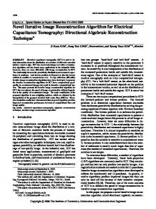
a) FM

b) x Gradient

c) y Gradient

d) z Gradient

Fig. 1 Field inhomogeneity map (in Hz) and its gradients (in Hz/cm) used in field inhomogeneity compensation. a) Field inhomogeneity map; Field inhomogeneity gradients: b) in xdirection, c) in y-direction, d) in z-direction. Some of the preliminary results are presented in this section. In this paper, we use a matrix size of 64x64 with 4 slices to test our implementation. Figure 1 shows one slice of the field inhomogeneity map and its gradients used in the image reconstruction. One can observe the presence of magnetic field inhomogeneity in the orbito-frontal cortex. Figure 2 a, c) shows reconstructions obtained without using the field map and its gradient; susceptibility artifacts such as

geometric distortion and signal loss are visible and degrade the reconstructed image. Figure 2 b, d) shows the CPU and GPU reconstructions obtained using our imaging model which compensated for susceptibility artifacts. From figure 2, we can see that CPU and GPU images are almost identical. The error (normalized root-mean-square error) between GPU and CPU is 2.94x10-4 without using SFU and 3.29x10-4 with using SFU. Therefore, we believe the error introduced by the SFU on the final result is acceptable.

a) CPU: no FM

b) CPU: FM

c) GPU: no FM

d) GPU: FM

Fig. 2 Image reconstruction comparisons between CPU and GPU. a) CPU: without FM compensation, b) CPU: with FM compensation, c) GPU: without FM compensation, d) GPU: with FM compensation. The GPU implementation has different performance versions by different optimization methods. For example, optimization methods include: storing voxel data in numerous processor registers to conserve memory bandwidth; placing data into constant memory to realize cached data access; tiling data based on the constant memory size; using hardware trigonometric functions, and so on. For simplicity, we provide the performance of two groups of optimization in GPU in this paper: with and without SFU (the rest optimizations are integrated inside both groups and their separate performance can be found in [15-17]). The optimization of CPU includes with and without paralleling code using multi-thread, etc. For compassion, the work is also tested in another pair of CPU and GPU. Table 1 represents the performance of different versions of CPU and GPU implementations with 8 iterations. So here we refer the tested processors as CPU1 (AMD Quad Core, 2.37 GHz), CPU2 (Intel Dual Core, 2.4 GHz) and GPU1 (G80), GPU2 (G280). The results in Table 1 show that the GPU computational performance up to 284x (with SFU) faster than the CPU with non-optimization, and 81x faster than the CPU with optimization. We believe this speedup of reconstruction is attractive to the clinical implementation. In addition, the proposed implementation of our imaging model on GPU can be easily extended to include spatially-varying smoothness constraints or other advanced applications to further improve the image quality.

Table. 1 Performance comparisons between CPU and GPU. GPU time Speedup CPU time

C P U

No Opt

CPU1 CPU2 CPU1

Opt CPU2

182 sec 130 sec 52 sec 69 sec

GPU No SFU

SFU

GPU1

GPU2

GPU1

GPU2

3.298 sec

1.529 sec

3.147 sec

0.640 sec

55X

119X

57X

284X

39X

85X

41X

203X

15X

34X

17X

81X

21X

45X

21X

107X

5. CONCLUSIONS We implement an advanced MR image reconstruction model on GPU using iterative conjugate gradients algorithm with magnetic field inhomogeneity compensation for geometric distortion and signal losses. The proposed GPU implementation speedups the image reconstruction around two orders of magnitude compared with CPU computation. And the error between CPU and GPU computation is negligible. This image reconstruction model could also be extend to include spatially-varying smoothness constraints, parallel MR imaging acquisition with multi-coil, and other advanced MR image reconstruction applications. As the result with this significant acceleration, accurate MR image reconstruction models will be able to meet the clinical and cognitive science requirements. Therefore, the MR image reconstruction will be able to improve both the image quality and reconstruction speed. ACKNWLWDGEMENT This work utilized the AC cluster [21] operated by the Innovative Systems Laboratory (ISL) at the National Center for Supercomputing Applications (NCSA). Special thanks to Jeremy Enos from ISL for his help with the system. REFERENCES [1] C.B. Ahn, J.H. Kim, Z.H. Cho. High-speed spiral-scan echo planar NMR imaging-I. IEEE Trans Med Imaging, 1986; 5(1): 2-7. [2] C.H. Meyer, B.S. Hu, D.G. Nishimura DG, A. Macovski. Fast spiral coronary artery imaging. Magn Reson Med, 1992 Dec; 28(2):202-13. [3] J.I. Jackson, C.H. Meyer, D.G. Nishimura, A. Macovski. Selection of a convolution function for Fourier inversion using gridding. IEEE Trans Med Imaging. 1991; 10(3): 473-8. [4] K. Sekihara, M. Kuroda, H. Kohno. Image restoration from non-uniform magnetic field influence for direct Fourier NMR imaging. Phys Med Biol. 1984 Jan; 29(1): 15-24. [5] D.C. Noll, C.H. Meyer, J.M. Pauly, D.G. Nishimura, A. Macovski. A homogeneity correction method for magnetic resonance imaging with time-varying gradients. IEEE Trans Med Imaging, 1991; 10(4): 629-637.

[6] B.P. Sutton, D.C. Noll, J.A. Fessler. Fast, iterative image reconstruction for MRI in the presence of field inhomogeneities. IEEE Trans Med Imaging, 2003 Feb; 22(2): 178–88. [7] D.C. Noll, J.A. Fessler, B.P. Sutton. Conjugate phase MRI reconstruction with spatially variant sample density correction. IEEE Trans Med Imaging, 2005 Mar; 24(3): 325-36. [8] J.A. Fessler, S. Lee, V.T. Olafsson, H.R. Shi, D.C. Noll. Toeplitz-based iterative image reconstruction for MRI with correction for magnetic field inhomogeneity. IEEE Trans Signal Process, 2005 Sep; 53(9): 3393-3402. [9] G. Liu, S. Ogawa. EPI image reconstruction with correction of distortion and signal losses. J Magn Reson Imaging. 2006 Sep; 24(3): 683-9. [10] B.P. Sutton, C. Ouyang, D.C. Karampinos, G.A. Miller. Current trends and challenges in MRI acquisitions to investigate brain function. Int J Psychophysiol. 2009 Jul; 73(1): 33-42. [11] J.R. Reichenbach, R. Venkatesan, D.A. Yablonskiy, M.R. Thompson, S. Lai, E.M. Haacke. Theory and application of static field inhomogeneity effects in gradient-echo imaging. J Magn Reson Imaging. 1997 Mar-Apr; 7(2): 266-79. [12] J.A. Fessler, D.C. Noll. Model-based MR Image Reconstruction with Compensation for Through-Plane Field Inhomogeneity. Proc. IEEE Intl. Symp. Biomed. Imag, 2007 April; 920-923 [13] B.P. Sutton, D.C. Noll, and J.A. Fessler, Compensating for within voxel susceptibility gradients in BOLD fMRI, Proc Int Soc Mag Res Med, 2004; 349. [14] Y. Zhuo, B.P. Sutton. Iterative Image Reconstruction Model Including Susceptibility Gradients Combined with Zshimming Gradients in fMRI. Proc IEEE Eng Med Biol Soc, Minneapolis, 2009 Sep; 5721-5724. [15] S.S. Stone, J.P. Haldar, S.C. Tsao, WmW. Hwu, Z.P. Liang, B.P. Sutton. Accelerating Advanced MRI Reconstructions on GPUs, J Parallel Distrib Comput. 2008 Oct; 68(10): 13071318. [16] S.S. Stone, H. Yi, J. P. Haldar, WmW. Hwu, B.P. Sutton, Z.P. Liang. How GPUs Can Improve the Quality of Magnetic Resonance Imaging, First workshop on General purpose processing on Graphics processing units (GPGPU), 2007 Oct. [17] WmW. Hwu, D. Nandakumar, J.P. Haldar, I.C. Atkinson, B.P. Sutton, Z.P. Liang, K.P. Thulborn. Accelerating MR Image Reconstruction on GPUs. Proc IEEE Intl. Symp. Biomed. Imag, 2009, June, 1283-1286. [18] J. Nickolls, I. Buck. NVIDIA CUDA software and GPU parallel computing architecture. Microprocessor Forum, 2007 May. [19] S. Ryoo, C. I. Rodrigues, S.S. Baghsorkhi, S.S. Stone, D.B. Kirk, WmW. Hwu. Optimization principles and application performance evaluation of a multithreaded GPU using CUDA. Symp Princ Practice Parallel Programming (PPOPP), 2008. [20] F. Wajer, K.P. Pruessmann. Major Speedup of Reconstruction for Sensitivity Encoding with Arbitrary Trajectories. Proc. 9th Intl. Soc. Mag. Reson. Med, 2001: 767. [21] V. Kindratenko, J. Enos, G. Shi, M. Showerman, G. Arnold, J. Stone, J. Phillips, WmW. Hwu, GPU Clusters for HighPerformance Computing, in Proc. Workshop on Parallel Programming on Accelerator Clusters, IEEE International Conference on Cluster Computing, 2009.