Accelerating Restore Performance of Data Deduplication ... - Usenix

ALACC: Accelerating Restore Performance of Data Deduplication Systems Using Adaptive Look-Ahead Window Assisted Chunk Caching Zhichao Cao, Hao Wen, Fenggang Wu, and David H.C. Du, Department of Computer Science, University of Minnesota, Twin Cities https://www.usenix.org/conference/fast18/presentation/cao

This paper is included in the Proceedings of the 16th USENIX Conference on File and Storage Technologies. February 12–15, 2018 • Oakland, CA, USA ISBN 978-1-931971-42-3

Open access to the Proceedings of the 16th USENIX Conference on File and Storage Technologies is sponsored by USENIX.

ALACC: Accelerating Restore Performance of Data Deduplication Systems Using Adaptive Look-Ahead Window Assisted Chunk Caching Zhichao Cao, Hao Wen, Fenggang Wu, and David H.C. Du Department of Computer Science, University of Minnesota, Twin Cities {caoxx380, wenxx159, wuxx0835, du}@umn.edu Abstract Data deduplication has been widely applied in storage systems to improve the efficiency of space utilization. In data deduplication systems, the data restore performance is seriously hindered by read amplification since the accessed data chunks are scattered over many containers. A container consisting of hundreds or thousands data chunks is the data unit to be read from or write to the storage. Several schemes such as forward assembly, container-based caching, and chunk-based caching are used to reduce the number of container-reads during the restore process. However, how to effectively use these schemes to get the best restore performance is still unclear. In this paper, we first study the trade-offs of using these schemes in terms of read amplification and computing time. We then propose a combined data chunk caching and forward assembly scheme called ALACC (Adaptive Look-Ahead Chunk Caching) for improving restore performance which can adapt to different deduplication workloads with a fixed total amount of memory. This is accomplished by extending and shrinking the look-ahead window adaptively to cover an appropriate data recipe range and dynamically deciding the memory to be allocated to forward assembly area and chunk-based caching. Our evaluations show the restore throughput of ALACC is higher than that of the optimum case of various configurations using the fixed amount of memory allocated to forward assembly and to chunkbased caching.

1

Introduction

Coming into the second decade of the twenty-first century, social media, cloud computing, big data, and other emerging applications are generating an extremely huge amount of data daily. Data deduplication is thus widely used in both primary and secondary storage systems to eliminate the duplicated data at chunk-level or file-level. In chunk-level data deduplication systems, the original data stream is segmented into data chunks and the du-

USENIX Association

plicated data chunks are eliminated (not to store). The original data stream is then replaced by an ordered list of references, called recipe, to the unique data chunks. A unique chunk is a new data chunk which has not appeared before. At the same time, only these unique data chunks are stored in the persistent storage. To maximize the I/O efficiency, instead of storing each single data chunk separately, these unique chunks are packed into containers based on the order of their appearances in the original data stream. A container which may consist of hundreds or thousands of data chunks is the basic unit of data read from or written to storage with a typical size of 4MB or larger. Restoring the original data is the reverse process of deduplication. Data chunks are accessed based on their indexing order in the recipe. The recipe includes the metadata information of each data chunk (e.g., chunk ID, chunk size, container address and offset). The corresponding data chunks are assembled in a memory buffer. Once the buffer is full, it will be sent back to the requesting client such that one buffer size data is restored. Requesting a unique or duplicate data chunk may trigger a container read if the data chunk is not currently available in memory, which causes a storage I/O and impacts restore performance. Our focus is specifically on restore performance in secondary storage systems. In order to reduce the number of container-reads, we may read ahead the recipe and allocate the data chunks to the buffers in the Forward Assembly Area (FAA). We can also cache the read-out container (containerbased caching) or a subset of data chunks (chunk-based caching) for future use. If a requested data chunk is not currently available in memory, it will trigger a containerread. It is also possible that only a few data chunks in the read-out container can be used in the current FAA. Therefore, to restore one container size of the original data stream, several more containers may have to be read from the storage causing read amplification. Read amplification causes low throughput and long completion time for the restore process. Therefore, the major goal of improving the restore performance is to reduce the number of container-reads [1]. For a given data stream, if

16th USENIX Conference on File and Storage Technologies

309

its deduplication ratio is higher, its read amplification is potentially more severe. There are several studies that address the restore performance issues [1, 2, 3, 4, 5, 6, 7]. The container-based caching scheme is used in [3, 4, 5, 7]. To use the memory space more efficient, a chunk-based LRU caching is applied in [1, 6]. In the restore, the sequence of future accesses is precisely recorded in the recipe. Using a look-ahead window or other methods can identify the future information to achieve a more effective caching policy. Lillibridge et al. [1] propose a forward assembly scheme. The proposed scheme reserves and uses multiple container size buffer in FAA to restore the data chunks with a look-ahead window which is the same size as FAA. Park et al. [7] use a fixed size look-ahead window to identify the cold containers and evict them first in a container-based caching scheme. The following issues are not fully addressed in the existing work. First, the performance and efficiency of container-based caching, chunk-based caching and forward assembly vary as the workload locality changes. When the total size of available memory for restore is fixed, how to use these schemes in an efficient way and make them adapt to the workload changing are very challenging. Second, how big is the look-ahead window and how to use the future information in the look-ahead window to improve the cache hit ratio are less explored. Third, acquiring and processing the future access information in the look-ahead window requires computing overhead. How to make better trade-offs to achieve good restore performance, but limit the computing overhead is also an important issue. To address these issues, in this paper we design a hybrid scheme which combines chunk-based caching and forward assembly. We also propose new ways of exploiting the future access information obtained in the lookahead window to make better decisions on which data chunks are to be cached or evicted. The sizes of the lookahead window, chunk cache, and FAA are dynamically adjusted to reflect the future access information in the recipe. In this paper, we first propose a look-ahead window assisted chunk-based caching scheme. A large LookAhead Window (LAW) provides the future data chunk access information to both FAA and chunk cache. Note that the first portion of the LAW (as the same size as that of FAA) is used to place chunks in FAA and the second part of the LAW is used to identify the caching candidates, evicting victims and accessing sequence of data chunks. We will only cache the data chunks that appear in the current LAW. Therefore, a cached data chunk is classified as either an F-chunk or a P-chunk. F-chunks are the data chunks that will be used in the near future (appear in the second part of LAW). P-chunks are the

310

data chunks that only appear in the first part of the LAW. If most of the cache space is occupied by the F-chunks, we may want to increase the cache space. If most of the cache space is occupied by P-chunks, caching is not very effective at this moment. We may consider to reduce the cache space or to enlarge the LAW. Based on the variation of the numbers of F-chunks, P-chunks, and other measurements, we then propose a self-adaptive algorithm (ALACC) to dynamically adjust the sizes of memory space allocated for FAA and chunk cache, and the size of LAW. If the number of F-chunks is low, ALACC extends the LAW size to identify more F-chunks to be cached. If the number of P-chunks is extremely high, ALACC either reduces the cache size or enlarges LAW size to adapt to the current access pattern. When the monitored measurements indicate that FAA performs better, ALACC increases the FAA size, thus reduces the chunk caching space, and gradually shrinks LAW. Since we consider a fixed amount of available memory, a reduction of chunk cache space will increase the same size of FAA or vice versa. For the reason that LAW only involves meta-data information which takes up a smaller data space, we ignore the space required by LAW, but focus more on the computing overhead caused by the operations of LAW in this paper. Our contributions can be summarized as follows: • We comprehensively investigate the performance trade-offs of container-based caching, chunk-based caching and forward assembly in different workloads and memory configurations. • We propose ALACC to dynamically adjust the sizes of FAA and chunk cache to adapt to the changing of chunk locality to get the best restore performance. • By exploring the cache efficiency and overhead of different LAW size, we propose and implement an effective LAW with its size dynamically adjusted to provide essential information for FAA and chunk cache and avoid unnecessary overhead. The rest of the paper is arranged as follows. Section 2 reviews the background of data deduplication and the current schemes of improving restore performance. Section 3 compares and analyzes different caching schemes. We first present a scheme with the pre-determined and fixed sizes of the forward assembly area, chunk cache, and LAW in Section 4. Then, the adaptive algorithm is proposed and discussed in Section 5. A brief introduction of the prototype implementation is in Section 6 and the evaluation results and analyses are shown in Section 7. Finally, we provide some conclusions and discuss the future work in Section 8.

16th USENIX Conference on File and Storage Technologies

USENIX Association

2

Background and Related Work

In this section, we first review the deduplication and restore process. Then, the related studies of improving restore performance are presented and discussed.

2.1

Data Deduplication Preliminary

Data deduplication is widely used in the secondary storage systems such as archiving and backup systems to improve the storage space utilization [8, 9, 10, 11, 12, 13, 14, 15]. Recently, data deduplication is also applied in the primary storage systems such as SSD array to make better trade-offs between cost and performance [16, 17, 18, 19, 20, 21, 22, 23]. To briefly summarize deduplication, as a data stream is written to the storage system, it is divided into data chunks, which are represented by a secure hash value called a fingerprint. The chunk fingerprints are searched in the indexing table to check their uniqueness. Only the new unique chunks are written to containers, and the original data stream is represented with a recipe consisting of a list of data chunk meta-information including the fingerprint. Restoring the original data stream back is the reverse process of deduplication. Starting from the beginning of the recipe, the restore engine identifies the data chunk meta-information sequentially, accesses the chunks either from memory or from storage, and assembles the chunks in an assembling buffer in memory. To get a chunk from storage to memory, the entire container holding the data chunk will be read, and the container may be distant from the last accessed container. Once the buffer is full, data is flushed out to the requested client. In the worst case, to assemble N duplicated chunks, we may need N container-reads. A straightforward solution to reduce the container-reads is to cache some of the containers or data chunks. Since some data chunks will be used very shortly after they are read into memory, these cached chunks can be directly copied from cache to the assembling buffer which can reduce the number of container-reads. Another way to reduce the number of container-reads is to store (re-write) some of the duplicated data chunks together with the unique chunks during the deduplication process in the same container. Therefore, the duplicated chunks and unique chunks will be read out together in the same container and thus avoids the needs of accessing these duplicated chunks from other containers. However, this approach will reduce the effectiveness of data deduplication.

2.2

Related Work on Restore Performance Improvement

Selecting and storing some duplicated data chunks during the deduplication process and designing efficient

USENIX Association

caching policies during the restore process are two major research directions to improve the restore performance. In the remaining of this subsection, we first review the studies of selectively storing the duplicated chunks. Then, we introduce the container-based caching, chunk-based caching and forward assembly. There have been several studies focusing on how to select and store the duplicated data chunks to improve the restore performance. The duplicated data chunks have already been written to the storage when they first appeared as unique data chunks and dispersed over different physical locations in different containers, which creates the chunk fragmentation issue [3]. During the restore process, restoring these duplicated data chunks causes potential random container-reads which lead to a low restore throughput. Nam et al. [3, 4] propose a way to measure the chunk fragmentation level (CFL). By storing some of the duplicated chunks to keep the CFL lower than a given threshold in a segment of the recipe, the number of container-reads is reduced. Kaczmarczyk et al. [2] use the mismatching degree between the stream context and disk context of the chunks to make the decision of storing selected duplicated data chunks. The container capping is proposed by Lillibridge et al. [1]. The containers storing the duplicated chunks are ranked and the duplicated data chunks in the lower ranking containers are selected and stored again. In a historical-based duplicated chunk rewriting algorithm [5], the duplicated chunks in the inherited sparse containers are rewritten. Due to the fact that rewriting some selected duplicated data chunks again sacrifices the deduplication ratio and the selecting and rewriting can be applied separately during the deduplication process, we will consider only the restore process in this paper. Different caching policies are studied in [1, 2, 3, 4, 6, 7, 24, 25]. Kaczmarczyk et al. [2] and Nam et al. [3, 4] use container-based caching. Other than using recency to identify the victims in the cache, Park et al. [7] propose a future reference count based caching policy with the information from a fixed size look-head window. Belady’s optimal replacement policy can only be used in a container-based caching schema [5]. It requires extra effort to identify and store the replacement sequence during the deduplication. If a smaller caching granularity is used, a better performance can be achieved. Instead of caching containers, some of the studies directly cache data chunks to achieve higher cache hit ratio [1, 6]. Although container-based caching has lower operating cost, chunk-based caching can better filter out the data chunks that are irrelevant to the near future restore and better improve the cache space utilization. However, the chunk-based caching with LRU also has some performance issues. The historical based LRU may

16th USENIX Conference on File and Storage Technologies

311

ds 3 2.11 26

fail to identify data chunks in the read-in container which are not used in the past and current assembling buffers, but they will be used in the near future. This results in cache misses. To address this issue, a look-ahead window which covers a range of future accesses from the recipe can provide the crucial future access information to improve the cache effectiveness. A special fashion of chunk-based caching proposed by Lillibridge et al. is called forward assembly [1]. Multiple containers (say k) are used as assembling buffers called Forward Assembly Area (FAA) and a look-ahead window of the same size is used to identify the data chunks to be restored in the next k containers. FAA can be considered as a chunk-based caching algorithm. It caches all the data chunks that appear in the next k containers and evicts any data chunk which does not appear in these containers. Since data chunks are directly copied from container-read buffer to FAA, it avoids the memory-copy operations from the container-read buffer to the cache. Therefore, forward assembly has lower overhead comparing with the chunk-based caching. Forward assembly can be very effective if each unique data chunk will reappear in a short range from the time it is being restored. As discussed, there is still a big potential to improve the restore performance if we effectively combine forward assembly and chunk-based caching using the future access information in the LAW. In this paper, we consider the total amount memory available to FAA and chunk cache is fixed. If the memory allocation for these two can vary according to the locality changing, the number of container-reads may be further reduced.

3

Analysis of Cache Efficiency

Before we start to discuss the details of our proposed design, we first compare and analyze the cache efficiency of container-based caching, chunk-based caching, and forward assembly. The observations and knowledge we learned will help our design. The traces used in the experiments of this section are summarized in Table 1. ds 1 and ds 2 are the last version of EMC 1 and FSL 1 traces respectively which are introduced in detail in Section 7.1. ds 3 is a synthetic trace based on ds 2 with larger re-use distance. The container size is 4MB. Computing time is used to measure the management overhead. It is defined as the total restore time excluding the storage I/O time which includes the cache adjustment time, memory-copy

312

300 250

Container_LRU Chunk_LRU Computing Time (seconds/GB)

ds 2 2.35 18

Container-reads per 100MB Restored

Table 1: Data Sets Data Set Name ds 1 Deduplication Ratio 1.03 Reuse Distance (# containers) 24

200 150 100 50 0

Container_LRU Chunk_LRU

5 4.5 4 3.5 3 2.5 2 1.5 1 0.5 0

Total Cache Size

Total Cache Size

(a) # Containers-reads per 100MB

(b) Computing time per 1GB re-

restored as cache size varies from 32MB to 1GB

stored as cache size varies from 32MB to 1GB

Figure 1: The cache efficiency comparison between chunk-based caching and container-based caching

time, CPU operation time, and others.

3.1

Caching Chunks vs. Caching Containers

Technically, caching containers can avoid the memory-copy from the container-read buffer to the cache. If the entire cache space is the same, the cache management overhead of container-based caching is lower than that of chunk-based caching. In most cases, some data chunks in a read-in container are irrelevant to the current and near-future restore process. Containerbased caching still caches these chunks and wastes the valuable memory space. Also, some of the useful data chunks are forced to be evicted together with the whole container which increases the cache miss ratio. Thus, without considering managing overhead, caching chunks can achieve better cache hit ratio than caching containers if we apply the same cache policy in most workloads. This is especially true if we use LAW as a guidance of future accesses. Only in the extreme cases that most data chunks in the container are used very shortly and there is very high temporal based locality, the cache hit ratio of caching containers can be better than that of caching chunks. We use the ds 2 trace to evaluate and compare the number of container-reads and the computing overhead of caching chunks and caching containers. We implemented the container-based caching and chunk-based caching with the same LRU policy. The assembling buffer used is one container size. As shown in Figure 1(b), the computing time of restoring 1GB data of caching chunks is about 15-150% higher than that of caching containers. Theoretically, the LRU cache insertion, lookup and eviction are O(1) time complexity. However, the computing time drops in both designs as the cache size increases. The reason is that with larger memory size more containers or data chunks can be cached and the cache eviction happens less frequently. There will be fewer memory-copy of containers or data chunks, which leads to less computing time.

16th USENIX Conference on File and Storage Technologies

USENIX Association

Forward Assembly

chunk_caching

Forward Assembly Rrestore Throughput (MB/S)

Computing Time (seconds/GB)

5 4 3 2 1 0 ds_1

ds_2

ds_3

(a) Computing time per 1GB restored

chunk_caching

38 37 36 35 34 33 32 31 30 29 ds_1

ds_2

ds_3

(b) Restore throughput

Figure 2: The cache efficiency comparison between forward assembly and chunk-based caching

Also, due to fewer cache replacements in the container-based caching, the computing time of caching containers drops quicker than that of caching chunks. However, as shown in Figure 1(a), the number of container-reads of caching chunks is about 30-45% fewer than that of caching containers. If one container-read needs 30ms, about 3% fewer container-reads can cover the extra computing time overhead of caching chunks. Therefore, caching chunks is preferred in the restore process, especially when the cache space is limited.

3.2

Forward Assembly vs. Caching Chunks

Comparing with chunk-based caching, forward assembly does not have the overhead of cache replacement and the overhead of copying data chunks from containerread buffer to the cache. Thus, the computing time of forward assembly is much lower than that of chunk-based caching. As for the cache efficiency, the two approaches have their own advantages and disadvantages with different data chunk localities. If most of the data chunks are unique or the chunk re-use locality is high in a short range (e.g., within the FAA range), forward assembly performs better than chunk-based caching. In this scenario, most of the data chunks in the read-in containers will only be used to fill the current FAA. In the same scenario, if chunk-based caching can intelligently choose the data chunks to be cached based on the future access information in LAW, it can achieve a similar number of container-reads but it has larger computing overhead. If the re-use distances of many duplicated data chunks are out of the FAA range, chunk-based caching performs better than forward assembly. Since these duplicated data chunks could not be allocated in the FAA, extra container-reads are needed when restoring these data chunks via forward assembly. In addition, a chunk in the chunk cache is only stored once while in forward assembly it needs to be stored multiple times in its appearing locations in the FAA. Thus, chunk-based caching can potentially cover more data chunks with larger re-use distances. When the managing overhead is less than the

USENIX Association

time saved by the reduction of container-reads, chunkbased caching performs better. We use the aforementioned three traces to compare the efficiency of forward assembly with that of chunk-based caching. The memory space used by both schemes is 64MB. For chunk-based caching, it uses the same size LAW as FAA to provide the information of data chunks accessed in the future. It caches the data chunks that appear in the LAW first, then adopts the LRU as its caching policy to manage the rest of caching space. As shown in Figure 2(a), the computing time of forward assembly is smaller than that of chunk-based caching. The restore throughput of forward assembly is higher than that of chunk based caching except in ds 3 as shown in Figure 2(b). In ds 3, the re-use distances of 77% of the duplicated data chunks are larger than the FAA range. More cache misses occur in forward assembly, while chunkbased caching can effectively cache some of these data chunks. In general, if the deduplication ratio is extremely low or most of the chunk re-use distances can be covered by the FAA, the performance of forward assembly is better than that of chunk-based caching. Otherwise, chunk-based caching can be a better choice.

4

Look-Ahead Window Assisted Chunkbased Caching

As discussed in the previous sections, combining forward assembly with chunk-based caching can potentially adapt to various workloads and achieve better restore performance. In this section, we design a restore algorithm with the assumption that the sizes of FAA, chunk cache and LAW are all fixed. We call the memory space used by chunk-based caching chunk cache. We first discuss how the FAA, chunk-based caching and LAW cooperate together to restore the data stream. Then, a detailed example is presented to better demonstrate our design. FAA consists of several container size memory buffers and they are arranged in a linear order. We call each container size buffer an FAB. A restore pointer pinpoints the data chunk in the recipe to be found and copied to its corresponding location in the first FAB at this time. The data chunks before the pointer are already assembled. Other FABs are used to hold the accessed data chunks if these chunks also appeared in these FABs. LAW starts with the first data chunk in the first FAB (FAB1 in the example) and covers a range bigger than that of FAA in the recipe. In fact, the first portion of the LAW (equivalent to the size of FAA) is used for the forward assembly purpose and the remaining part of LAW is used for the purpose of chunk-based caching. An assembling cycle is the process to completely restore the first FAB in the FAA. That is, the duration after the previous first FAB is written back to the client

16th USENIX Conference on File and Storage Technologies

313

Look-Ahead Window Covered Range Restored 22

2

8

22 18

2

5

Information for Chunk Cache

Unknown

10 14 10 15 17 22 18 23 12 13 32 23 28

6

……

FAA Covered Range

……

restore

Restored Data 22

2

8

22

FAA 18

2

5

FAB1

10

10

=

FAB2

……

Container Read Buffer 10 12 13 17

Client

Persistent Storage

Chunk Cache High Priority End 18

10

22

5

12

2

13

8

F-cache P-cache Low Priority End

Figure 3: An example of look-ahead window assisted chunk-based caching

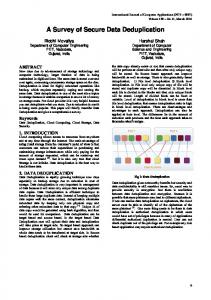
and a new empty FAB is added to the end of FAA to the time when the new first FAB is completely filled up. At the end of one assembling cycle (i.e., the first FAB is completely assembled), the content of the FAB is written back to the requested client as the restored data and this FAB is removed from the FAA. At the same time, a new empty FAB will be added to the end of the FAA so that FAA is maintained with the same size. For the LAW, the first portion (one container size) corresponding to the removed FAB is dropped and one more segment of recipe (also one container size) is appended to the end of LAW. Then, the restore engine starts the next assembly cycle to fill in the new first FAB of the current FAA. During the assembling cycle, the following is the procedure of restoring the data chunk pointed by the restore pointer. If the data chunk at the restore pointer has already been stored by previous assembling operations, the pointer will be directly moved to the next one. If the data chunk has not been stored at its location in the FAB, the chunk cache is checked first. If the chunk is found in the cache, the data chunk is copied to the locations where this data chunk appears in all the FABs including the location pointed by the restore pointer. Also, the priority of the chunk in the cache is adjusted accordingly. If the chunk is not in the chunk cache, the container that holds the data chunk will be read in from the storage. Then, each data chunk in this container is checked with LAW to identify all the locations it appears in the FAA. Then, the data chunk is copied to the corresponding locations in all FABs if they exist. Next, we have to decide which chunks in this container are to be inserted to the chunk cache according to a caching policy, and it will be described later. After this data chunk is restored, the restore pointer moves to the next data chunk in the recipe. The read-in container will be replaced by the next requested container. An example is shown in Figure 3, and it will be described in detail in the last part of this section.

314

When inserting data chunks from the read-in container to the chunk cache, we need to identify the potential usage of these chunks in the LAW and treat them accordingly. Based on the second portion of LAW (i.e., the remaining LAW after the size of FAA), the data chunks from the read-in container can be classified into three categories: 1) U-chunk (Unused chunk) is a data chunk that does not appear in the current entire LAW, 2) P-chunk (Probably used chunk) is a data chunk that appears in the current FAA but does not appear in the second portion of the LAW, and 3) F-chunk (Future used chunk) is a data chunk that will be used in the second portion of the LAW. Note that a F-chunk may or may not be used in the FAA. F-chunks are the data chunks that should be cached. If more cache space is still available, we may cache some P-chunks according to their priorities. That is, F-chunks have priority over P-chunks for caching. However, each of them has a different priority policy. The priority of F-chunks is defined based on the ordering of their appearance in the second portion of the LAW. That is, an F-chunk to be used in the near future in the LAW has a higher priority over another F-chunk which will be used later in the LAW. The priority of P-chunks is LRU based. That is, the most recently used (MRU) P-chunk has a higher priority over the least recently used P-chunks. Let us denote the cache space used by F-chunks (P-chunks) as F-cache (P-cache). The boundary between the F-cache and P-cache is dynamically changing as the number of F-chunks and that of P-chunks vary. When the LAW advances, new F-chunks are added to the F-cache. An F-chunk that has been restored and no longer appeared in the LAW will be moved to the MRU end of the P-cache. That is, this chunk becomes a Pchunk. The priorities of some F-chunks are adjusted according to their future access sequences. The new Pchunks are added to the P-cache based on the LRU order of their last appearance. Some P-chunks may become F-chunks if they appear in the newly added portion of LAW. When the cache eviction happens, data chunks are evicted from the LRU end of the P-cache first. If there is no P-chunk in P-cache, eviction starts from the lowest priority end of the F-cache. Figure 3 is an example to show the entire working process of our design. Suppose one container holds 4 data chunks. The LAW covers the data chunks of 4 containers in the recipe from chunk 18 to chunk 28. The data chunks before the LAW have been assembled and written back to the client. The data chunks beyond the LAW is unknown to the restore engine at this moment. There are two buffers in the FAA denoted as FAB1 and FAB2. Each FAB has a size of one container and also holds 4 data chunks. FAA covers the range from chunk 18 to chunk 17. The rest information of data chunks in the LAW (from chunk 22 to chunk 28) are used for the chunk

16th USENIX Conference on File and Storage Technologies

USENIX Association

5

The Adaptive Algorithm

The performance of the look-ahead window assisted chunk-based caching is better than that of simply combining the forward assembly with LRU-based chunk caching. However, the sizes of FAA, chunk cache and LAW are pre-determined and fixed in this design. As discussed in the previous sections, FAA and chunk cache have their own advantages and disadvantages for different workloads. In fact, in a given workload like a backup trace, most data chunks are unique at the beginning. Later in different sections of the workload, they may have various degrees of duplication and re-usage. Therefore, the sizes of FAA and chunk cache can be dynamically changed to reflect the locality of the current section of a workload. It is also important to figure out what the appropriate LAW size is to get the best restore performance given a configuration of the FAA and chunk cache. We propose an adaptive algorithm called

USENIX Association

40

14

35

12

Computing Time (seconds/GB)

Restore Throughput (MB/S)

cache. The red frames in the figure show the separations of data chunks in containers. The labeled chunk number represents the chunk ID and is irrelevant to the order of the data chunk appearing in the recipe. In FAB1, chunks 18, 2, 5 have already been stored and the current restore pointer is at data chunk 10 (pointed by the red arrow). This data chunk has neither been allocated nor been cached. The container that stores chunk 10, 12, 13 and 17 is read out from the storage to the container read buffer. Then, the data of chunk 10 is copied to the FAB1. At the same time, chunk 10 also appears in the FAB2 and the chunk is stored in the corresponding position too. Next, the restore pointer moves to the chunk 14 at the beginning of the FAB2. Since FAB1 has been fully assembled, its content is written out as restored data and it is removed from FAA. The original FAB2 becomes the new FAB1 and a new FAB (represented with dotted frames) is added after FAB1 and becomes the new FAB2. All the data chunks in the container read buffer are checked with the LAW. Data chunk 10 is used in the FAA but it does not appear again in the rest of LAW. So chunk 10 is a P-chunk and it is inserted to the MRU end of the P-cache. Chunk 12 and chunk 13 are not used in the current FAA but they will be used in the next two assembling cycles within the LAW. They are identified as F-chunks and added to the F-cache. Notice that chunk 12 appears after chunk 22 and chunk 13 is used after chunk 12 as shown in the recipe. Therefore, chunk 13 is inserted into the low priority end and chunk 12 has the priority higher than chunk 13. Chunk 17 has neither been used in the FAA nor appeared in the LAW. It is a U-chunk and it will not be cached. When restoring chunk 14, a new container will be read into the container read buffer and it will replace the current one.

30 25 20 15 10 5

10 8 6 4 2 0

0 12

24

48

96

192 384 768

Look Ahead Window size (# of containers)

(a) Restore throughput

12

24

48

96

192 384 768

Look Ahead Window Size (# of containers)

(b) Computing time per 1GB restored

Figure 4: The restore performance and computing overhead variation as the LAW size increases ALACC that can dynamically adjust the sizes of FAA, chunk cache and LAW according to the workload variation during the restore process. First, we evaluate and analyze the restore performance of using different LAW sizes. Then, we present the details of ALACC.

5.1

Performance Impact of LAW Size

We did an experiment that varies the LAW sizes for a given workload and compared the restore throughput and required computing overhead. We use an 8MB (2 container size) FAA and a 24MB (6 container size) chunk cache as the memory space configuration and increase the LAW size from 12 container size to 768 container size (it covers the original data stream size from 48MB to 3GB). As shown in Figure 4, the computing time continuously increases as the LAW size increases due to higher overhead to process and maintain the information in the LAW. When the size of LAW is larger than 96, the restore throughput starts to decrease. The performance degradation is caused by the increase of computing overhead and less efficiency of chunk cache. Thus, using an appropriate LAW size is important to make better trade-offs between cache efficiency and computing overhead. We can explain the observation by analyzing the chunk cache efficiency. Suppose the LAW size is SLAW chunks, the FAA size is SFAA chunks, and the chunk cache size is Scache chunks. Note that we use a container size as the basic unit for allocation and the number of containers can be easily translated to the number of chunks. Assume one data chunk Ci is used at the beginning of the FAA and it will be reused after DCi chunks (i.e., the reuse distance of this chunk). If DCi < SFAA , it will be reused in the FAA. If SFAA < DCi , this chunk should be either an Fchunk or a P-chunk. However, the chunk category highly depends on the size of SLAW . If the LAW only covers the FAA range (SFAA = SLAW < DCi ), the proposed algorithm degenerates to the LRU-based chunk caching algorithm. If SFAA < DCi < SLAW , we can definitely identify this chunk as an F-chunk and decide to cache this chunk. However, if SLAW < DCi , this chunk will be identified as

16th USENIX Conference on File and Storage Technologies

315

a P-chunk and it may or may not be cached (this depends on the available space in cache). Therefore, at least we should ensure SFAA + Scache ≤ SLAW . If the LAW size is large enough and most of the chunk cache space are occupied by F-chunks, the cache efficiency is high. However, once the cache is full of Fchunks, the newly identified F-chunk may or may not be inserted into the cache. This depends on its reuse order. Thus, continuing increase the LAW size would not further improve the cache efficiency. What is worse, a larger LAW size requires more CPU and memory resources to identify and maintain the future access information. As we discuss before, if SLAW is the same as SFAA , all cached chunks are P-chunks and chunk caching becomes an LRU-based algorithm. Thus, the best trade-off between cache efficiency and overhead is when the total number of P-chunks is as low as possible but not 0. However, it may be hard to maintain the number of P-chunks low all the time, especially when there is a very limited number of F-chunks identified with a large LAW size. In this case, the size of LAW should not be extended or it should be decreased slightly.

5.2

ALACC

Based on the previous analysis, we propose an adaptive algorithm, which dynamically adjusts the memory space ratio of FAA and chunk cache, and the size of LAW. We apply the adjustment at the end of each assembling cycle right after the first FAB is restored. Suppose at the end of ith assembling cycle, the sizes of FAA, i i i chunk cache and LAW are SFAA , Scache and SLAW coni i tainer size respectively. SFAA + Scache is fixed. To avoid an extremely large LAW size, we set a maximum size of LAW (MaxLAW ) that is allowed during the restore. The algorithm of ALACC optimizes the memory allocation to FAA and chunk cache first. On one hand, if the workload has an extremely low locality or its duplicated data chunk re-use distance is small, FAA is preferred. On the other hand, according to the total number of P-chunk in the cache, the chunk cache size is adjusted. Then, according to the memory space allocation changing and the total number of F-chunk in the cache, the LAW size is adjusted to optimize the computing overhead. The detailed adjustment conditions and actions are described in the following part of this section. In our algorithm, the conditions of increasing the FAA size are examined first. If any of these conditions is satisfied, FAA will be increased by 1 container size and the size of chunk cache will be decreased by 1 container accordingly. Otherwise, we will check the conditions of adjusting the chunk cache size. Notice that the size of FAA and chunk cache could remain the same if none of the adjustment conditions are satisfied. Finally, the LAW size will be changed.

316

FAA and LAW Size Adjustment. As discussed in Section 3.2, FAA performs better than chunk cache when 1) the data chunks in the first FAB are identified mostly as unique data chunks and these chunks are stored in the same or close containers, or 2) the re-use distance of most duplicated data chunks in this FAB is within the FAA range. Regarding the first condition, we consider that the FAB can be filled in by reading in no more than 2 containers and none of the data chunks needed by the FAB is from the chunk cache. When this happens, we consider this assembling cycle FAA effective. For Condition 2, we observed that if the re-use distances of 80% or more of the duplicated chunks in this FAB is smaller than the FAA size, forward assembly performs better. Therefore, based on the observations, we use either of the following two conditions to increase the FAA size. First, if the number of consecutive FAA effective assembling cycles becomes bigger than a given threshold, we increase the FAA size by 1 container. Here, we use the i current FAA size, SFAA , as the threshold to measure this i condition at the end of ith assembling cycle. When SFAA size is small, the condition is easier to satisfy and the i size of FAA can be increased faster. When SFAA is large, the condition is more difficult to satisfy. After increasing the FAA size by one, the count of consecutive FAA effective assembling cycles is reset to 0. Second, the data chunks used during the ith assembling cycle to fill up the first FAB in FAA are examined. If the re-use distances of more than 80% of these examined chunks during the i ith assembling cycle are smaller than SFAA + 1 container size, the size of FAA will be increased by 1 container. i+1 i That is, SFAA = SFAA + 1. If the FAA size is increased by 1 container, the size of chunk cache will decrease by 1 container accordingly. i i Originally, SLAW − SFAA container size LAW information i is used by Scache container size cache. After the FAA i i adjustment, SLAW − SFAA + 1 container size LAW is used i by Scache − 1 container size cache, which wastes the information in the LAW. Thus, the LAW size is decreased by 1 container size to avoid the same size LAW used by a now smaller size chunk cache. After the new sizes of FAA, chunk cache and LAW are decided, two empty FABs (one to replace the re-stored FAB and the other reflects the increasing size of FAA) will be added to the end of FAA and the chunk cache starts to evict data chunks. Then, the (i + 1)th assembling cycle will start. Chunk Cache and LAW Size Adjustment. If there is no adjustment to the FAA size, we now consider the adjustment of chunk cache size. After finished the ith assembling cycle, the total number (NF−chunk ) of F-chunks in the F-cache and the total number (NP−chunk ) of Pchunks in the P-cache are counted. Also, the number of F-chunks that are newly added to the F-cache during the ith assembling cycle is denoted by NF−added . These

16th USENIX Conference on File and Storage Technologies

USENIX Association

newly added F-chunks either come from the read-in containers in the ith assembling cycle or are transformed from P-chunks due to the extending of the LAW. We examine the following three conditions. First, if NP−chunk becomes 0, it indicates that all the cache space is occupied by F-chunks. The current LAW size is too large and the number of F-chunks based on the current LAW is larger than the chunk cache capacity. Therefore, the chunk cache size will be increased by 1 container. Meanwhile, the size of LAW will decrease by 1 container to reduce the unnecessary overhead. Second, if the total size of NF−added is bigger than 1 container, it indicates that the total number of F-chunks increases very quickly. Thus, we increase the chunk cache size by 1 container and decrease LAW by 1 container. Notice that a large NF−added can happen when NP−chunk is either small or large. This condition will make our algorithm quickly react to the changing of the workload. Third, if NP−chunk is very large (i.e., NF−chunk is very small), the chunk cache size will be decreased by 1 container. In this situation, the LAW size is adjusted differently according to either of the following two conditions: 1) In the current workload, there are few data chunks in the FAB that are reused in the future, and 2) The size of LAW is too small, it cannot look ahead far enough to find more F-chunks for the current workload. For Condition 1, we decrease the LAW size by 1 container. For Condition 2, we increase the LAW size by K containers. Here, K is calculated by K = i i i (MaxLAW − SLAW )/(SFAA + Scache ). If LAW is small, its size is increased by a larger amount. If LAW is big, its size will be increased slowly.

6

Prototype Implementation

We implemented a prototype of a deduplication system (a C program with 11k LoC) with several restore designs: FAA, container-based caching, chunk-based caching, LAW assisted chunk-based caching, and ALACC. For the deduplication process, it can be configured to use different container size and chunk size (fixed size chunking and variable size chunking) to process the real world data or to generate deduplication traces. To satisfy the flexibility and efficiency requirements of ALACC, we implemented several data structures. All the data chunks in the chunk cache are indexed by a hashmap to speed up the searching operation. F-chunks are ordered by their future access sequence provided by the LAW and P-chunks are indexed by an LRU list. The LAW maintains the data chunk metadata (chunk ID, size, container ID, address and offset in the container) in the same order as they are in the recipe. Although the insertion and deletion in the LAW is O(1) by using the hashmap, identifying the F-chunk priority is O(log(N)), where N is the LAW size. A Restore Recovery Log (RRL) is maintained to ensure reliability. When one FAB is full and flushed out, the chunk ID of the last chunk in the FAB, the chunk location in the recipe, the restored data address, FAA, chunk cache and LAW configurations are logged to the RRL. If the system is down, by using the information in the RRL, the restore process can be recovered to the latest restored cycle. The FAA, chunk cache and LAW will be initiated and reconstructed.

7

Performance Evaluation

LAW Size Independent Adjustment If none of the aforementioned conditions are satisfied (the sizes of FAA and chunk cache remain the same), the LAW size will be adjusted independently. Here, we use the NF−chunk to decide the adjustment. If NF−chunk is smaller than a given threshold (e.g., 20% of the total chunk cache size), the LAW size will be slightly increased by 1 container to process more future information. If NF−chunk is higher than the threshold, the LAW size will be decreased by 1 to reduce the computing overhead.

To comprehensively evaluate our design, we implement five restore engines including ALACC, LRU-based container caching (Container LRU), LRU-based chunk caching (Chunk LRU), forward assembly (FAA), and fixed combination of forward assembly and chunk-based caching. However, in the last case, we show only the Optimal Fix Configuration (Fix Opt). Fix Opt is obtained by exhausting all possible fixed combinations of FAA, chunk cache, and LAW sizes.

ALACC makes the trade-offs between computing overhead and the reduction of container-reads, such that a higher restore throughput can be achieved. Instead of using a fixed value as the threshold, we tend to dynamically change FAA size and LAW size. It can slow down the adjustments when the overhead is big (when the LAW size is large) and it can speed up the adjustment when the overhead is small to quickly reduce the container-reads (when FAA size is small).

The prototype is deployed on a Dell PowerEdge R430 server with a 2.40GHz Intel Xeon with 24 cores and 32GB of memory using Seagate ST1000NM00339ZM173 SATA hard disk with 1TB capacity as the storage. The container size is configured as 4MB. All five implementations are configured with one container size space as container read buffer and memory size of S containers. Container LRU and Chunk LRU use one container for FAA and S − 1 for container or chunk cache.

USENIX Association

7.1

Experimental Setup and Data Sets

16th USENIX Conference on File and Storage Technologies

317

Dataset Size ACS1 DR2 CFL3 1 2

FSL 2 317.4GB 4KB 4.88 3.3

EMC 1 29.2GB 8KB 1.04 14.7

EMC 2 28.6GB 8KB 4.8 19.3

ACS stands for Average Chunk Size DR stands for the Deduplication Ratio, which is the original data size divided by the deduplicated data size. CFL stands for the Chunk Fragmentation Level, which is the average number of containers that stores the data chunks from one container size of original data stream. High CFL value leads to low restore performance.

Table 3: The FAA/chunk cache/LAW configuration (# of containers) of Fix Opt for each deduplication trace FSL 1 FSL 2 EMC 1 EMC 2 Size 4/12/56 6/10/72 2/14/92 4/12/64 18 17 16 15 14 13 2 4

FAA Size

3

FSL 1 103.5GB 4KB 3.82 13.3

FAA uses LAW of S container size and all S memory space as the forward assembly area. The specific configuration of Fix Opt is given in Section 7.2. In all experiments, ALACC is initiated with S/2 container size FAA, S/2 container size chunk cache and 2S container size LAW before the execution. For the reason that ALACC requires to maintain at least one container size space as FAB, the FAA size varies from 1 to S and the chunk cache size varies from (S − 1) to 0 accordingly. After one version of backup is restored, the cache is cleaned. We use four deduplication traces in the experiments as shown in Table 2. FSL 1 and FSL 2 are two different backup traces from FSL /home directory snapshots of the year 2014 [26]. Each trace has 6 full snapshot backups and the average chunk size is 4KB. EMC 1 and EMC 2 are the weekly full-backup traces from EMC and each trace has 6 versions and 8KB average chunk size [27]. EMC 1 was collected from an exchange server and EMC 2 was the /var directory backup from a revision control system. To measure the restore performance, we use the speed factor, computing cost factor and restore throughput as the metrics. The speed factor (MB/container-read) is defined as the mean data size restored per container read. Higher speed factors indicate higher restore performance. The computing cost factor (second/GB) is defined as the time spent on computing operations (subtracting the storage I/O time from the restore time) per GB data restored and the smaller value is preferred. The restore throughput (MB/second) is calculated from the original data stream size divided by the total restore time. We run each test 5 times and present the mean value. Notice that, for the same trace using the same caching policy, if the restore machine and the storage are different, the computing cost factor and restore throughput can be different while the speed factor is the same.

318

Restore Throughput (MB/S)

Table 2: Characteristics of datasets

12 6 8 10 12 14

96

88

80

72

12-13

64

13-14

48 56 LAW Size

14-15

40

32

15-16

24

16

16-17

17-18

Figure 5: The restore throughput of different FAA, chunk cache and LAW size configurations

7.2

Optimal Performance of Fixed Configurations

In LAW assisted chunk-based caching design, the sizes of FAA, chunk cache and LAW are fixed and are not changed during the restore process. To find out the best performance of a configuration for a specific trace with a given memory size, in our experiments we run all possible configurations for each trace to discover the optimal throughput. This optimal configuration is indicated by Fix Opt. For example, for 64MB memory, we vary the FAA size from 4MB to 60MB and the chunk cache size from 60MB to 4MB. At the same time, the LAW size increases from 16 containers to 96 containers. Each test tries one set of fixed configuration and finally, we draw a three-dimensional figure to find out the optimal results. An example is shown in Figure 5, for FSL 1, the optimal configuration has 4 containers of FAA, 12 containers of chunk cache and a LAW size of 56 containers. One throughput peak is when the LAW is small. The computing cost is low while the container-reads are slightly higher. The other throughput peak is when the LAW is relatively large. With more future information, the container-reads are lower but the computing cost is higher. The optimal configuration of each trace is shown in Table 3, the sizes of FAA and chunk cache can be calculated by the number of containers times 4MB.

7.3

Restore Performance Comparison

Using the same restore engine and storage as discovering the Fix Opt, we evaluate and compare the speed fac-

16th USENIX Conference on File and Storage Technologies

USENIX Association

Computing Cost Factor

1 0.8 0.6 0.4 0.2

20 16 12 8 4

1

2 3 4 Version Number

0

5

(a) Speed factor of FSL 1 Container_LRU FAA ALACC

2 3 Version Number

4

Computing Cost Factor

4 3 2 1 0

12

Container_LRU FAA ALACC

2 3 Version Number

4

6 4 2 0

2 1.5 1 0.5 0 1 2 3 Version Number

4

4

1.5 1 0.5 2 3 Version Number

4

Chunk_LRU Fix_Opt

2

3 2 1 0

Container_LRU FAA ALACC

2 3 Version Number

(j) Speed factor of EMC 2

4

5

5

Container_LRU FAA ALACC

Chunk_LRU Fix_Opt

40 30 20 10 0 0

60

1

2 3 Version Number

4

5

Container_LRU FAA ALACC

Chunk_LRU Fix_Opt

50 40 30 20 10 0 0

5

1

2 3 Version Number

4

5

(i) Restore throughput of EMC 1

Chunk_LRU Fix_Opt

1.6 1.2 0.8 0.4

105

Container_LRU FAA ALACC

Chunk_LRU Fix_Opt

90 75 60 45 30 15 0

0 1

4

(f) Restore throughput of FSL 2

2

1

2 3 Version Number

50

Chunk_LRU Fix_Opt

2.5

0

1

60

(h) Computing cost factor of EMC 1

4

0

70

5

0

5

Computing Cost Factor

5

Container_LRU FAA ALACC

3

(g) Speed factor of EMC 1 Container_LRU FAA ALACC

0

(e) Computing cost factor of FSL 2

2.5

0

1 2 3 Version Number

Chunk_LRU Fix_Opt

Computing Cost Factor

3

5

(c) Restore throughput of FSL 1

8

(d) Speed factor of FSL 2 Container_LRU FAA ALACC

10

Chunk_LRU Fix_Opt

10

5

Chunk_LRU Fix_Opt

15

0

Restore Throughput (MB/S)

1

Container_LRU FAA ALACC

20

5

0 0

25

(b) Computing cost factor of FSL 1

Chunk_LRU Fix_Opt

5 Speed Factor

1

Restore Throughput(MB/S)

0

Speed Factor

Chunk_LRU Fix_Opt

0

0

Speed Factor

Container_LRU FAA ALACC

Restore Throughput(MB/S)

Speed Factor

1.2

Chunk_LRU Fix_Opt

Restore Throughput(MB/S)

Container_LRU FAA ALACC

0

1

2 3 Version Number

4

(k) Computing cost factor of EMC 2

5

0

1

2 3 Version Number

4

5

(l) Restore throughput of EMC 2

Figure 6: The restore performance results comparison of Container LRU, Chunk LRU, FAA, Fix Opt and ALACC. Notice that the speed factor, computing cost factor and restore throughput vary largely in different traces, we use different scales among subfigures to show the relative improvement or difference of the five designs in the same trace.

USENIX Association

16th USENIX Conference on File and Storage Technologies

319

Table 4: The percentage of memory size occupied by FAA of ALACC in each restore testing case Version # 0 1 2 3 4 5 FSL 1 50% 38% 39% 38% 40% 38% FSL 2 67% 67% 64% 69% 64% 57% 26% 24% 14% 17% 16% 16% EMC 1 EMC 2 7% 8% 8% 8% 8% 7%

Table 5: The average LAW size (# of ALACC in each restore testing case Version # 0 1 2 3 FSL 1 31.2 30.5 31.4 32.2 FSL 2 44.6 44.1 40.1 32.3 77.1 83.1 88.7 84.2 EMC 1 EMC 2 95.3 95.2 95.1 95.3

tor, computing cost and restore performance (throughput) of the four traces with 64MB total memory. The evaluation results are shown in Figure 6. As indicated in Table 2, the CFL of FSL 2 is much lower than the others, which leads to a very close restore performance of all the restore designs. However, when the CFL is high, ALACC is able to adjust the sizes of FAA, chunk cache, and LAW to adapt to the highly fragmented chunk storing, and achieves higher restore performance. The computing cost varies in different traces and versions. In most cases, the computing cost of FAA is relatively lower than the others, because it avoids the cache insertion, look-up, and eviction operations. As expected, the computing overhead of Chunk LRU is usually higher than that of Container LRU due to more management operations for smaller caching granularity. However, in EMC 2, the computing overhead of Container LRU is much higher than the other four designs. The overhead is caused by the high frequent cache replacement and extremely high cache miss ratio. The cache miss ratio of Container LRU is about 3X higher than that of Chunk LRU. The time of reading containers from storage to the read-in buffer dominates the restore time. Thus, the speed factor can nearly determine the restore performance. Comparing the speed factor and restore throughput of the same trace, for example, trace FS 1 in Figure 6(a) and 6(c), the curves of the same cache policy are very similar. For all 4 traces, the overall average speed factor of ALACC is 83% higher than Container LRU, 37% higher than FAA, 12% higher than Chunk LRU and 2% higher than Fix Opt. The average computing cost of ALACC is 27% higher than that of Container LRU, 23% higher than FAA, 33% lower than Chunk LRU and 26% lower than Fix Opt. The average restore throughput of ALACC is 89% higher than that of Container LRU, 38% higher than FAA, 14% higher than Chunk LRU and 4% higher than Fix Opt. In our experiments, the speed factor of ALACC is higher than those of Container LRU, Chunk LRU, and FAA. More importantly, ALACC achieves at least a similar or better performance as Fix Opt. By dynamically adjusting the sizes of FAA, chunk cache and LAW, the improvement of the restore throughput is higher than the speed factor. Notice that we

need tens of experiments to find out the optimal configurations of Fix Opt which is almost impossible to carry out in a real-world production scenario. The main goal of ALACC is to make better tradeoffs between the number of container-reads and the required computing overhead. The average percentage of the memory space occupied by FAA of ALACC is shown in Table 4 and the average LAW size is shown in Table 5. The percentage of chunk cache in the memory can be calculated by (1 − FAA percentage). The mean FAA size and LAW size vary largely in different workloads. The restore data with larger data chunk re-use distance usually needs smaller FAA size, larger cache size, and larger LAW size, like in traces FSL 1, FSL 2, and EMC 2. One exception is trace EMC 1. This trace is very special, only about 4% data chunks are duplicated chunks and they are scattered over many containers. The performances of Container LRU, Chunk LRU and FAA are thus very close since extra container-reads will always happen when restoring the duplicated chunks. By adaptively extending the LAW to a larger size (about 80 containers and 5 times larger than FAA cover range) and using larger chunk cache space, ALACC successfully identifies the data chunks that will be used in far future and caches them. Therefore, ALACC can outperform others in such an extreme workload. Assuredly, ALACC has the highest computing overhead (about 90% higher than others in average) as shown in Figure 6(h). Comparing the trend of varying FAA and LAW sizes of Fix Opt (shown in Table 3) with that of ALACC (shown in Tables 4 and 5), we can find that ALACC usually applies smaller LAW and larger cache size than Fix Opt. Thus, ALACC achieves lower computing cost and improves the restore throughput as shown in Figures 6(b), 6(e) and 6(k). In EMC 2, ALACC has a larger cache size and a larger LAW size than those of Fix Opt. After we exam the restore log, we find that the P-chunks occupied 95% the cache space in more than 90% of the assembling cycles. A very small portion of data chunks is duplicated many times, which can explain why the Chunk LRU performs close to Fix Opt. In such an extreme case, ALACC makes the decision to use a larger cache space and a larger LAW size such that it can still adapt to the workload and maintain a high speed factor

320

16th USENIX Conference on File and Storage Technologies

containers) of 4 32.0 32.8 76.1 94.8

5 30.7 36.9 82.6 95.2

USENIX Association

P-chunks per container

’FSL_2_v1.log’ using 14

1000 800 600 400 200 0

0

500

1000

1500

2000

2500

Asssemble cycle number

3000

FAA size

(a) P-chunk numbers per container size chunk cache 16 14 12 10 8 6 4 2 0

’FSL_2_v1.log’ using 4

0

500

1000

1500

2000

2500

Asssemble cycle number

3000

Cache size

(b) FAA size (# of containers) 16 14 12 10 8 6 4 2 0

’FSL_2_v1.log’ using 5

8 0

500

1000

1500

2000

2500

Asssemble cycle number

LAW Size

100

’FSL_2_v1.log’ using 6

80 60 40 20 0

500

1000

1500

2000

Asssemble cycle number

2500

3000

(d) LAW size (# of containers)

Figure 7: The variation of P-chunk numbers per container size chunk cache, FAA size, chunk cache size, and LAW size during the restore of FSL 1 in version 0 and high restore throughput as shown in Figures 6(j) and 6(l). In general, ALACC successfully adapts to the locality changing and delivers high restore throughput for a given workload.

7.4

Conclusion and Future Work

3000

(c) Chunk cache size (# of containers)

0

1500), most of the chunk cache space is occupied by the P-chunks and there are few duplicated data chunks. Thus, ALACC uses a larger FAA and a smaller LAW. If the number of P-chunk is relatively low, more caching space is preferred. For example, in the assembling cycle range (700–900), the number of P-chunks is lower than 200 (i.e., more than 80% of the chunk cache space is used for F-chunks). As expected, the FAA size drops quickly and the chunk cache size increases sharply and stays at a high level. Meanwhile, since the cache space is increased, the LAW size is also increased to cover larger recipe range and to identify more F-chunks. In general, ALACC successfully monitors the workload variation and self-adaptively reacts to the number of Pchunks variation as expected, and thus, delivers higher restore throughput without manual adjustments.

Improving restore performance of deduplication system is very important. In this paper, we studied the effectiveness and the efficiency of different caching mechanisms applied to the restore process. Based on the observations of the caching efficiency experiments, we design an adaptive algorithm called ALACC which is able to adaptively adjust the sizes of the FAA, chunk cache and LAW according to the workload changes. By making better trade-offs between the number of containerreads and computing overhead, ALACC achieves much better restore performance than container-based caching, chunk-based caching and forward assembly. In our experiments, the restore performance of ALACC is slightly better than the best performance of restore engine with all possible configurations of fixed sizes of FAA, chunk cache and LAW. In our future work, duplicated data chunk rewriting will be investigated and integrated with ALACC to further improve the restore performance of data deduplication systems for both primary and secondary storage systems.

The Adaptive Adjustment in ALACC

To verify the adaptive adjustment process of ALACC, we write the log at the end of each assembling cycle and using P-chunk as an example to show the size adjustment of FAA, chunk cache and LAW by ALACC. The log records the P-chunk numbers per container size cache , the sizes of FAA, chunk cache, and LAW. We use FSL 2 version 1 as an example and the results are shown in Figure 7. The number of P-chunks per container size cache is very low at the beginning and varies sharply as assembly cycle increases as shown in Figure 7(a). One container size cache can store about 1000 data chunks in average. During the assembling cycle range (1000–

USENIX Association

Acknowledgments We thank all the members in CRIS group to provide the useful comments to improve our design. We thank Dongchul Park for assistance with the trace exploring and pre-processing, and Baoquan Zhang for the specific reviewing comments. We would like to thank our shepherd, Philip Shilane, for his useful comments and suggestions. This work is partially supported by the following NSF awards: 1305237, 1421913, 1439622 and 1525617.

16th USENIX Conference on File and Storage Technologies

321

References [1] Mark Lillibridge, Kave Eshghi, and Deepavali Bhagwat. Improving restore speed for backup systems that use inline chunk-based deduplication. In 11th USENIX Conference on File and Storage Technologies (FAST 13), pages 183–198, 2013. [2] Michal Kaczmarczyk, Marcin Barczynski, Wojciech Kilian, and Cezary Dubnicki. Reducing impact of data fragmentation caused by in-line deduplication. In Proceedings of the 5th Annual International Systems and Storage Conference, page 15. ACM, 2012. [3] Youngjin Nam, Guanlin Lu, Nohhyun Park, Weijun Xiao, and David HC Du. Chunk fragmentation level: An effective indicator for read performance degradation in deduplication storage. In High Performance Computing and Communications (HPCC), 2011 IEEE 13th International Conference on, pages 581–586. IEEE, 2011.

[9] Wei Zhang, Tao Yang, Gautham Narayanasamy, and Hong Tang. Low-cost data deduplication for virtual machine backup in cloud storage. In HotStorage, 2013. [10] Fanglu Guo and Petros Efstathopoulos. Building a high-performance deduplication system. In 2011 USENIX Annual Technical Conference (USENIX ATC 11), 2011. [11] Min Fu, Dan Feng, Yu Hua, Xubin He, Zuoning Chen, Wen Xia, Yucheng Zhang, and Yujuan Tan. Design tradeoffs for data deduplication performance in backup workloads. In 13th USENIX Conference on File and Storage Technologies (FAST 15), pages 331–344, 2015. [12] Jaehong Min, Daeyoung Yoon, and Youjip Won. Efficient deduplication techniques for modern backup operation. IEEE Transactions on Computers, 60(6):824–840, 2011.

[4] Young Jin Nam, Dongchul Park, and David HC Du. Assuring demanded read performance of data deduplication storage with backup datasets. In Modeling, Analysis & Simulation of Computer and Telecommunication Systems (MASCOTS), 2012 IEEE 20th International Symposium on, pages 201–208. IEEE, 2012.

[13] Deepavali Bhagwat, Kave Eshghi, Darrell DE Long, and Mark Lillibridge. Extreme binning: Scalable, parallel deduplication for chunk-based file backup. In Modeling, Analysis & Simulation of Computer and Telecommunication Systems, 2009. MASCOTS’09. IEEE International Symposium on, pages 1–9. IEEE, 2009.

[5] Min Fu, Dan Feng, Yu Hua, Xubin He, Zuoning Chen, Wen Xia, Fangting Huang, and Qing Liu. Accelerating restore and garbage collection in deduplication-based backup systems via exploiting historical information. In USENIX Annual Technical Conference (USENIX ATC 14), pages 181–192, 2014.

[14] Sean Quinlan and Sean Dorward. Venti: A new approach to archival storage. In 1st USENIX Conference on File and Storage Technologies (FAST 02), volume 2, pages 89–101, 2002.

[6] Bo Mao, Hong Jiang, Suzhen Wu, Yinjin Fu, and Lei Tian. Sar: Ssd assisted restore optimization for deduplication-based storage systems in the cloud. In Networking, Architecture and Storage (NAS), 2012 IEEE 7th International Conference on, pages 328–337. IEEE, 2012.

[15] Cezary Dubnicki, Leszek Gryz, Lukasz Heldt, Michal Kaczmarczyk, Wojciech Kilian, Przemyslaw Strzelczak, Jerzy Szczepkowski, Cristian Ungureanu, and Michal Welnicki. Hydrastor: A scalable secondary storage. In 7th USENIX Conference on File and Storage Technologies (FAST 09), volume 9, pages 197–210, 2009.

[7] Dongchul Park, Ziqi Fan, Young Jin Nam, and David HC Du. A lookahead read cache: Improving read performance for deduplication backup storage. Journal of Computer Science and Technology, 32(1):26–40, 2017.

[16] Kiran Srinivasan, Timothy Bisson, Garth R Goodson, and Kaladhar Voruganti. idedup: latencyaware, inline data deduplication for primary storage. In 10th USENIX Conference on File and Storage Technologies (FAST 12), volume 12, pages 1– 14, 2012.

[8] Benjamin Zhu, Kai Li, and R Hugo Patterson. Avoiding the disk bottleneck in the data domain deduplication file system. In 6th USENIX Conference on File and Storage Technologies (FAST 08), volume 8, pages 1–14, 2008.

[17] Wenji Li, Gregory Jean-Baptise, Juan Riveros, Giri Narasimhan, Tony Zhang, and Ming Zhao. Cachededup: in-line deduplication for flash caching. In 14th USENIX Conference on File and Storage Technologies (FAST 16), pages 301–314, 2016.

322

16th USENIX Conference on File and Storage Technologies

USENIX Association

[18] Biplob K Debnath, Sudipta Sengupta, and Jin Li. Chunkstash: Speeding up inline storage deduplication using flash memory. In USENIX annual technical conference (USENIX ATC 10), 2010. [19] Yoshihiro Tsuchiya and Takashi Watanabe. Dblk: Deduplication for primary block storage. In Mass Storage Systems and Technologies (MSST), 2011 IEEE 27th Symposium on, pages 1–5. IEEE, 2011. [20] Vasily Tarasov, Deepak Jain, Geoff Kuenning, Sonam Mandal, Karthikeyani Palanisami, Philip Shilane, Sagar Trehan, and Erez Zadok. Dmdedup: Device mapper target for data deduplication. In 2014 Ottawa Linux Symposium, 2014. [21] Sonam Mandal, Geoff Kuenning, Dongju Ok, Varun Shastry, Philip Shilane, Sun Zhen, Vasily Tarasov, and Erez Zadok. Using hints to improve inline block-layer deduplication. In 14th USENIX Conference on File and Storage Technologies (FAST 16), pages 315–322, 2016. [22] Zhuan Chen and Kai Shen. Ordermergededup: Efficient, failure-consistent deduplication on flash. In 14th USENIX Conference on File and Storage Technologies (FAST 16), pages 291–299, 2016. [23] Ahmed El-Shimi, Ran Kalach, Ankit Kumar, Adi Ottean, Jin Li, and Sudipta Sengupta. Primary data deduplication-large scale study and system design. In 2012 USENIX Annual Technical Conference (USENIX ATC 12), pages 285–296, 2012. [24] Ziqi Fan, David HC Du, and Doug Voigt. H-arc: A non-volatile memory based cache policy for solid state drives. In Mass Storage Systems and Technologies (MSST), 2014 30th Symposium on, pages 1–11. IEEE, 2014. [25] Ziqi Fan, Fenggang Wu, Dongchul Park, Jim Diehl, Doug Voigt, and David HC Du. Hibachi: A cooperative hybrid cache with nvram and dram for storage arrays. In Mass Storage Systems and Technologies (MSST), 2017 IEEE 33th Symposium on. IEEE, 2017. [26] http://tracer.filesystems.org/. [27] Nohhyun Park and David J Lilja. Characterizing datasets for data deduplication in backup applications. In Workload Characterization (IISWC), 2010 IEEE International Symposium on, pages 1– 10. IEEE, 2010.

USENIX Association

16th USENIX Conference on File and Storage Technologies

323