Acceleration of an Improved Retinex Algorithm Yuan-Kai Wang* and Wen-Bin Huang Department of Electrical Engineering, Fu Jen Catholic University, 510, Zhongzheng Rd., Xinzhuang Dist., New Taipei County 24205, Taiwan *
[email protected]
algorithm is very high. However, how to reduce the complexity and use the massively parallel architecture and hierarchical memory to improve the efficiency is a focus of the study. The General-Purpose computation on Graphics Processing Units (GPGPUs) [4] have evolved into multithreads and many-core processors that are especially well-suited to data parallel computation. Another important capability is software-programmable that enables users to easily develop parallel algorithms in program-level parallelism. The Compute Unified Device Architecture (CUDA) can be used to achieve the high parallelism in this platform. GPGPU/CUDA has many properties that are suitable for real-time image/video processing. Therefore, parallelization of the Retinex algorithms by GPGPU should greatly improve its performance. The purpose of this paper is to accelerate the Retinex algorithm that is called GPURetinex algorithm which is a data parallel algorithm based on GPGPU/CUDA. A preliminary data parallel algorithm has been proposed to parallelize the Retinex algorithm on GPGPU [5]. The previous method can achieve good performance speedup to 43 times that does not include the time of data transfer and memory management. However, more detail analysis shows that the algorithm can be further improved by optimizing memory usage and out-of-boundary extrapolation in the convolution step, especially reduce the number of cache miss and divergent branch. In addition, we found that the previous algorithm may produce satisfied results only for low-dynamic-range images, but not for images of high dynamic range, low-key, and uneven illumination. Therefore, a parallel histogram stretching method is devised in this paper to enhance the algorithm for more challenging problem.
Abstract Retinex is an image restoration method and the center/surround Retinex is appropriate for parallelization because it utilizes a convolution operation with large kernel size to achieve dynamic range compression and color/lightness rendition. However, its great capability for image enhancement comes with intensive computation. This paper presents a GPURetinex, which is a data parallel algorithm based on GPGPU/CUDA. The GPURetinex exploits GPGPU’s massively parallel architecture and hierarchical memory to improve efficiency. The GPURetinex has been further improved by optimizing the memory usage and out-of-boundary extrapolation in the convolution step. In our experiments, the GPURetinex can gain 72 times speedup compared with the optimized single-threaded CPU implementation by OpenCV for the images with 2048 x 2048 resolution. The proposed method also outperforms a Retinex implementation based on the NPP (nVidia Performance Primitives).
1. Introduction The Retinex algorithm is an effective method to remove environmental light interference and is used as a preprocessing step in many computer vision algorithms. Land [1] first conceived the idea of the Retinex and has a variety of extensions. The Retinex algorithms can be classified into three classes: path-based algorithms, recursive algorithms, and center/surround algorithms. Among the three classes, the center/surround Retinex algorithm has no iterative process and is suitable for parallelization. Single Scale Retinex (SSR) [2] algorithm is the first proposed center/surround algorithm that can either achieve dynamic range compression or color/lightness rendition, but not both simultaneously. The dynamic range compression and color/lightness rendition were combined by the Multi-Scale Retinex (MSR) and Multi-Scale Retinex with Color Restoration (MSRCR) [3] algorithms with a universally applied color restoration. The Retinex algorithm contains the computing of center/surround information, a log-domain processing, and normalization. The time complexity of the Retinex
2. Background In this section, we will review the computational model of Retinex algorithms and the parallelization of vision algorithms by GPGPU’s many-core capability.
2.1. Computational Model of Retinex Algorithms The center/surround Retinex algorithm was first proposed by Land [6]. The new technique allows each pixel 72
where ri(x,y) is the color restoration coefficient in the i th spectral band, N the number of spectral bands(N = 3 for typical RGB color images), β is a gain constant, and α controls the strength of nonlinearity. However, if the color restoration factor ri(x,y) is not considered, then Ri(x,y) becomes the MSR output and has some drawbacks for color images [7]. Furthermore, if both the color restoration factor ri(x,y) is not considered and the number of center/surround function n is 1, then Ri(x,y) becomes the SSR output.
being treated only once and selected sequentially. New pixel values are obtained by computing the ratio between each treated pixel and a weighted average of its surrounding area. Rahman et al. [2] utilized a Gaussian blur operation to compute the center/surround information and the method is called SSR. The MSR is an extension of SSR and offers the combining of the dynamic range compression and color/lightness rendition by averaging three SSRs of different spatial scales. The MSRCR was proposed to compensate for the loss of color saturation inherently by a color restoration factor. The center/surround Retinex algorithms are faster than the path-based ones, and the amount of parameters is greatly reduced. It has lower computational cost and overcomes the deficiency of the recursive Retinex algorithm. In addition, the Retinex algorithms of the path and recursive classes can not be parallelized effectively due to the algorithmic characteristics of high data dependency among sequential steps, while the Retinex algorithm of the center/surround class can be greatly parallelized. Therefore, the center/surround Retinex algorithm is suitable for GPGPU/CUDA implementation. Next, we will introduce the MSRCR, MSR, and SSR with a unified view. The basic form of MSRCR is given in Eq.(1). n
(
)
Ri ( x, y ) = ri ( x, y ) × ∑ Wk log Ii ( x, y ) − log ⎡⎣ Fk ( x, y ) ⊗ Ii ( x, y ) ⎤⎦ , k =1
2.2. Parallel Processing by GPGPU’s Multicore Recently, GPGPUs have evolved to programmable multicore architecture and become the focus of much research in parallel and high performance computing. Owens et al. [8] gave a broad survey of general-purpose computation on graphics hardware. There are a lot of implementations using GPGPU/CUDA to accelerate computationally intensive tasks in image processing and computer vision domains. A parallel Canny edge detector under CUDA was demonstrated [9], including all stages of algorithms. They achieved 3.8 times speedup on the images with 3936 x 3936 resolution compared to an optimized OpenCV version. A real-time 3D visual tracker with an efficient Sparse-Template-based particle filtering was implemented by Lozano and Otsuka [10]. Their implementation can achieve 10 times performance improvements compared to a similar CPU-only tracker. Wang and Huang [5] proposed a GPU method for Retinex and the speedup can achieve 43 times. Further speedup up to 72 times is obtained in this paper by incorporating an 8-bit/pixel data format, a transpose operation, a CUDA array usage, and hardware support for the out-of-boundary extrapolation in the convolution step.
(1)
where Ri(x,y) is the MSRCR output at the coordinates (x,y), Ii(x,y) the original image, Fk the kth center/surround function, Wk the weight of Fk, n the number of center/surround functions, and “ ⊗ ” denotes the 2D convolution operation. The center/surround function Fk (x,y) is given in Eq.(2). − ⎛⎜ x2 + y 2 ⎞⎟
Fk ( x, y ) = Ke
⎝
⎠
ck 2
,
(2)
where ck is the kth Gaussain center/surround scale(smaller value of ck leads to narrower surround and larger value of ck leads to wider surround), and K is a constant satisfying the ∫∫ F ( x, y )dxdy = 1 .
3. The GPURetinex Method An overview of the GPURetinex is shown in Figure 1. The GPURetinex uses the heterogeneous programming model provided by CUDA, where the serial code segments are executed on the host (CPU) and only the parallel code segments are executed on the device (GPU). The host loads an original image and performs the memory transfer of the image from host to device. Then five steps, including Gaussain blur, log-domain processing, reduction, normalization, and histogram stretching, are parallelly executed with Single Program Multiple Data (SPMD) model in the GPGPU. The final step is to transfer the result from device to host. It is very important for the computing of the Gaussian blur in the GPURetinex to adopt the separable convolution kernel can reduce computation time [5]. We further improve the memory usage and adopt the automatic mirror
The Eq.(1) uses multiple center/surrounds and different weights to achieve a graceful balance between dynamic range compression and tonal rendition. The MSRCR usually adopts a combination of three scales representing narrow, medium, and wide center/surrounds to simultaneously achieve both dynamic range compression and tonal rendition. The color restoration factor ri(x,y) in Eq.(1) is considered to offer color constancy. The color restoration factor ri(x,y) is given in Eq.(3). ⎛ ⎞ ⎜ I i ( x, y ) ⎟ ⎟ , ri ( x, y ) = β × log ⎜ α × N (3) ⎜ ⎟ I ( x , y ) ∑ i ⎜ ⎟ i =1 ⎝ ⎠
73
addressing to support the out-of-boundary extrapolation. For the memory usage, an 8-bit/pixel image format and a transpose operation are adopted to reduce the cache miss in hierarchical memory access. The CUDA arrays which are opaque memory layouts optimized for texture fetching and support four out-of-boundary extrapolations is also adopted. We adopt the automatic mirror addressing to implement the Gaussian blur in order to reduce the divergent branch which costs many computations in hardware. The computing of the Gaussian blur in the GPURetinex will be divided into the convolutions of row filter and column filter. The convolution is illustrated in Figure 2. The data distribution of the parallel Gaussian blur convolution adopts a horizontal stripe method. Details can be found in [5].
The next step is the parallel computing of log-domain processing, as indicated in Eq.(1). These computations can be performed in parallel at pixel-wise level and are shown in Figure 3. The GPURetinex adopts three Gaussian blur images with different scales to combine the effects of dynamic range compression and color/lightness rendition. Three Gaussian blur images with different scales are respectively denoted as G1(x,y), G2(x,y), and G3(x,y). The I(x,y) and R(x,y) are the input and output images. The data distribution in this step uses the horizontal stripe method. Each thread block contains 256 threads (T0~T255) and the total number of thread blocks is 120. Each thread computes the operations for all pixels within its horizontal stripe subimage. GPU
… B119 B0 Height = 256
Width = 256
T255
…
B119 B0 Height = 256
R(x,y)
…
…
Parallel Histogram Stretching
G3(x,y)
T1: R(1,0) = r(1,0)*exp (W1 *(log (I(1,0) +1)-log(G1 (1,0)+1))+ … W2 *(log (I(1,0) +1)-log(G2 (1,0)+1))+ W3 *(log (I(1,0) +1)-log(G3 (1,0)+1)))
T0T1
…
Copy Data from GPGPU to CPU
G2(x,y)
…
Global Memory
B0 B1
Parallel Normalization
G1(x,y)
B15 Width = 256
T0: R(0,0) = r(0,0)*exp(W1 *(log (I(0,0) +1)-log(G 1(0,0)+1))+ W2*(log (I(0,0) +1)-log(G 2(0,0)+1))+ W3*(log (I(0,0) +1)-log(G 3(0,0)+1)))
Parallel Reduction
T255
…
B15
B119 B0 Height = 256
…
…
Parallel Log-domain Processing
I(x,y)
B0 B1
…
Parallel Gaussian Blur
B0 B1
T0T1
…
GPGPU
T255
…
CPU Copy Data from CPU to GPGPU
T0T1
B15 Width = 256
Figure 1. Overview of the GPURetinex.
Global Memory
Figure 3. The parallel computing of log-domain processing. GPU SrcImage
Row Filter m1 m2 m3
S1 S2 S3
T0 T1 o1 o2
…
TempImage Block 0 Block 1
T 255
Compared with the square subimage method implemented in [5], this pixel-wise implementation has the same efficiency but is more intuitive. Next we have to enhance the result obtained by the Retinex processing. There are two methods for the enhancement: normalization and histogram stretching. Normalization method expands the compressed dynamic range of Ri ( x, y ) into [0, 255]. The formula is given in Eq.(4).
…
Constant Memory
…
256
256
Block 255 256
Texture Memory
256
T0: o 1 = S1 * m1 + S1 * m2 + S2 * m3 T1: o 2 = S1 * m1 + S2 * m2 + S3 * m3
Global Memory
…
T255
⎛ 255 N i ( x, y ) = [ Ri ( x, y ) − min i ] × ⎜ max i − min i ⎝
(a) GPU TempImage
Column Filter m1 m2 m3
S1 S2 S3
T0 T1 o1 o2
…
DstImage Block 0 Block 1
T 255
… 256
Block 255 256
Texture Memory
256
Global Memory
…
T0: o 1 = S1 * m1 + S1 * m2 + S2 * m3 T1: o 2 = S1 * m1 + S2 * m2 + S3 * m3
(4)
where N i ( x, y ) is the output in the i th spectral band. Ri ( x, y ) is the results of log-domain processing in Eq.(1). The maxi and mini are maximum and minimum values in the i th spectral band. A parallel reduction method is utilized to find the two extreme values. A detail description is referred to [5]. However, the Retinex output can not sometimes gain the best color/lightness rendition and contrast after the processing of normalization, especially for images of high dynamic range, low-key, and uneven illumination. The histogram stretching which uses histogram of N i ( x, y ) is adopted to gain the best color/lightness rendition and
…
Constant Memory
256
⎞ ⎟, ⎠
T255
(b) Figure 2. The blur convolution in the GPURetinex. (a) Row filtering. (b) Column filtering.
74
contrast. The concept of the histogram stretching is shown in Figure 4. The h(i) is the histogram and aˆmin and aˆmax are two desired extreme values. The aˆmin is statistically
merge histograms of per-warp into one and write to partial histogram in the global memory. The second step of the parallel histogramming is to merge the partial histogram into a global histogram. In the step, the total number of thread blocks is 256 and each thread block sums a bin of global histogram from the partial histogram. The reads of each thread block are uncoalesced, but this step takes only a fraction of total processing time. When a thread block writes all values of a bin in the partial histogram into its shared memory, many recursive doubling procedures is executed to merge all values of a bin into one.
obtained by a predefined quantile plow that is defined as the percentage of pixels with gray levels less than aˆmin . aˆmax is also defined with a quantile phigh in a similar way. The values aˆmin and aˆmax can be obtained from the image’s cumulative histogram [11] H(i), as shown in Eq.(5) and Eq.(6).
aˆmin = min {i | H (i ) ≥ M ⋅ N ⋅ plow } ,
}
aˆmax = max i | H (i ) ≤ M ⋅ N ⋅ (1 − phigh ) ,
T0
(6)
GPU
N(x,y) T 255 … B0 … B1
T0 T1
…
{
(5)
where 0 ≤ plow , phigh ≤ 1 , plow + phigh ≤ 1 , and M ⋅ N is the
PartialHistograms …
B239 B0
T255
…
…
number of pixels in the image N i ( x, y ) . The f (a) is given in Eq.(7). ⎧0 , if a ≤ aˆmin ⎪ 255 ⎪ f (a) = ⎨( a − aˆmin ) × , if aˆmin < a < aˆmax . (7) ˆ amax − aˆmin ⎪ ⎪ 255 , if a ≥ aˆmax ⎩ The upper and lower quantiles can be set to the same value, plow = phigh = p , with p ∈ [0.005, 0.015] .
B0 B1
240
…
B239 256
1024
Global Memory
B63 1024
Step1
Global Memory
Step2
PartialHistograms B255 … B0 B1
T0 T1
T0 T1 … …
Shared Memory 240
T 239
Bin 0
0
1
… T 255 2
127 128 129 130
255
3 2 1 … 3 2 2 6 … 0
B0
256 Global Memory
Figure 5. The parallel histogramming in the GPURetinex.
h(i)
aˆ min plow
0
amin
Finally, the cumulative histogram H(i), aˆmin and aˆmax are computed sequentially from the small data array h(i), and the stretching in Eq.(7) is performed in parallel on a pixel-wise level. The horizontal stripe method is used in this stretching step for the data distribution. Each thread block that contains 256 threads (T0~T255) and the total number of thread blocks is 120. Each thread computes the operation in Eq.(7) for a pixel within its horizontal stripe subimage.
aˆ max phigh
amax
i
a f (a) 0
255
Figure 4. The histogram stretching.
4. Experimental Results About one hundred color images were tested in our experiments to verify the enhancement results of the GPURetinex. Since no difference of execution time is revealed in the experimental images, only three example images are chosen for the following discussions. The performance of GPURetinex has been tested on Tesla C1060 and CUDA 3.2. The GPGPU is cooperated with an Intel Core2 Duo of 3.0GHz. For comparison purposes, a serial implementation of Retinex was developed and run with single thread on one core of the CPU. The Gaussian blur filtering in the CPU version adopts the optimized implementation in the OpenCV library. Figure 6 (a)(d)(g) give the three original images. The first image is an indoor scene of non-uniform illumination. The second image is an outdoor scene of low-key with loss
The parallelization of the above histogram stretching method includes two steps: parallel histogramming to get h(i), and parallel stretching to perform Eq.(7). The parallel histogramming in the GPURetinex is shown in Figure 5. The histogramming can be divided into two steps. The first step of the parallel histogramming is to count the pixels of N(x,y) in parallel into a partial histogram. In the step, the data distribution belongs to the horizontal stripe method. Each thread block that contains 256 threads (256 * 1 as the dimension of the thread block: T0~T255) and the total number of thread blocks is 240. Each warp of a thread block has its local histogram in shared memory. Each thread of a warp uses the shared memory atomic addition function to sum the local histogram. Then the next step is to
75
of color and detail in the shadow. The third image is a scene of high dynamic range with strong sunlight and dark shadow. Figure 6 (b)(e)(h) are the enhanced results of GPURetinex_N with no histogram stretching, that is the previous parallel Retinex algorithm [5]. Figure 6 (c)(f)(i) are the enhanced results of the GPURetinex with histogram stretching. We can see the best results that using additional histogram stretching method has the best color/lightness rendition and contrast. We next compare the execution time of the GPURetinex method with other algorithms. Three Gaussian filters of widths 17, 83, and 253 are adopted to compute the center/surround information in the experiments. The detailed execution times are shown in Table 1. The "GPU_P" columns represent the previous parallel Retinex algorithm in [5]. The "Others" columns include the time of memory management and transfer time. For CPU it is only the cost of memory management, while for GPU it includes not only memory management but also the data transfer. Figure 7 illustrates total execution time between the GPU and CPU versions of Retinex. The total execution time of both CPU and GPU versions increases proportionally with respect to image dimensions. In addition, the versions with histogram stretching just cost a little time than the versions with no histogram stretching. The GPURetinex_N is 1.5 times faster than the GPURetinex_P on average. We also adopt the NPP [12] library v3.2 (functions: nppiFilterRow_8u_C1R and nppiFilterColumn_8u_C1R) to implement the Gaussian blur due to the Gaussian blur step always consumes the most processing time. The GPURetinex is 1.5 times faster than the GPURetinex_NPP on average. In addition, the NPP v3.2 functions do not support out of border extrapolation and make the result of Retinex incorrectly. Figure 8 shows the speedup of GPU version over CPU version. The speedup is measured using the total execution time that does not include the cost of memory management and data transfer. The speedup of each algorithm in Figure 8 has a peak on this platform. This means that each line will tend to its peak gradually with the increase of image dimensions. In addition, the "Speedup" is lower than the "Speedup_N" for each image resolution. This is due to the speedup of histogramming step is lower. For the image of 2048 x 2048 resolution, the GPURetinex can gain 72x speedup compared with CPURetinex, the GPURetinex_N is 1.7 times faster than the GPURetinex_P, the GPURetinex is 1.7 times faster than the GPURetinex_NPP. The experimental results of the GPU-accelerated Retinex demonstrate excellent speed boost.
the Retinex algorithm. A parallel histogram stretching is devised to gain the best color rendition and contrast. Although using histogram stretching costs additional time than the versions with no histogram stretching, the color rendition and contrast is better. Moreover, the GPURetinex is further improved by optimizing the memory usage and hardware support of out-of-boundary extrapolation in the convolution step to gain better performance. Our experimental results show that using the GPGPU/CUDA can greatly accelerate the Retinex algorithm and the GPURetinex can gain 72 times speedup compared with the CPU-based implementation on the images with 2048 x 2048 resolution.
Acknowledgment This work was supported financially by the Ministry of Economic Affairs under Project No. MOEA 99-EC-17-A-02-S1-032 in Technology Development Program for Academia.
References [1] E. Land. The Retinex. Amer. Scient., 52(2):247–264, 1964. [2] D. J. Jobson, Z. Rahman, and G. A. Woodell. Properties and performance of a center/surround retinex. IEEE Trans. on Image Processing, 6(3):451-462, 1997. [3] D. J. Jobson, Z. Rahman, and G. A. Woodell. A multi-scale Retinex for bridging the gap between color images and the human observation of scenes. IEEE Trans. on Image Processing, 6(7):965-976, 1997. [4] S. Ryoo, C. I. Rodrigues, S. S. Baghsorkhi, S. S. Stone, D. B. Kirk, and W. W. Hwu. Optimization principles and application performance evaluation of a multithreaded GPU using CUDA. In Proc. 13th ACM SIGPLAN Symp., Salt Lake City, Utah, USA, 73-82, 2008. [5] Y. K. Wang and W. B. Huang. Acceleration of the Retinex algorithm for image restoration by GPGPU/CUDA. In Proc. IS&T/SPIE Electronic Imaging, San Francisco, California, USA, 7872:78720E-78720E-11, 2011. [6] E. Land. An alternative technique for the computation of the designator in the retinex theory of color vision. In Proc. National Academy of Science, USA, 83:3078-3080, 1986. [7] L. Tao and V. Asari. Modified luminance based MSR for fast and efficient image enhancement. In 32nd Applied Imagery Pattem Recognition, Washington, DC, USA, 174-179, 2003. [8] J. D. Owens, D. Luebke, N. Govindaraju, M. Harris, J. Krger, A. E. Lefohn, and T. J. Purcell. A survey of general-purpose computation on graphics hardware. Computer Graphics Forum, 26(1):80–113, 2007. [9] Y. Luo and R. Duraiswami. Canny edge detection on NVIDIA CUDA. In Proc. CVPR, Anchorage, AK, 1-8, 2008 [10] M. Lozano and K. Otsuka. Real-time visual tracker by stream processing. J. of Sign. Process. Syst., 57(2):674–679, 2008. [11] W. Burger and M. J. Burge. Digital Image Processing: An Algorithmic Introduction using java. Springer, 2008. [12] NVIDIA Performance Primitives. http://developer.nvidia.com/npp
5. Conclusions This paper presents a GPU-accelerated data parallel algorithm called GPURetinex that is proposed to parallelize
76
(a)
(b)
(c)
(d)
(e)
(f)
(g) (h) (i) Figure 6. The three sets of original and enhanced images. (a) The first image, (d) the second image, (g) the third image, (b)(e)(h) the results of GPURetinex_N, (c)(f)(i)the results of GPURetinex. Table 1. Execution times of six parts in the Retinex algorithm with respect to image resolutions. Image Size 256 x 256 512 x 512 1024 x 1024 2048 x 2048
Gaussian Blur Log-domain Processing Reduction Normalization Histogramming Stretching Total Execution Time Others CPU GPU_P GPU CPU GPU_P GPU CPU GPU_P GPU CPU GPU_P GPU CPU GPU_P GPU CPU GPU_P GPU CPU GPU_P GPU CPU GPU_P GPU 139.12 5.31 3.67 63.03 0.38 0.34 1.13 0.44 0.20 2.20 0.10 0.09 1.18 0.52 2.85 0.07 209.51 6.23 4.89 0.28 3.31 4.95 593.27 18.45 12.37 251.83 0.75 0.78 4.55 0.44 0.20 8.80 0.15 0.14 5.68 0.63 11.27 0.12 875.40 19.79 14.24 1.11 12.95 13.31 2415.06 77.89 47.64 1005.19 2.67 3.10 18.70 0.57 0.30 35.76 0.34 0.36 22.60 1.10 44.49 0.35 3541.80 81.47 52.85 4.75 42.65 45.49 11094.30 343.03 195.09 4011.22 10.51 14.61 74.62 1.45 0.74 142.85 1.20 1.21 84.14 3.43 167.92 1.49 15575.05 356.19 216.57 19.23 163.87 166.92
80
100000
70 60
1000
Speedup
Time(msec)
10000
100 10 1
50 40 30 20
256 x 256
512 x 512
1024 x 1024
2048 x 2048
CPURetinex_N
205.48
858.45
3474.71
15322.99
CPURetinex
209.51
875.40
3541.80
15575.05
GPURetinex_P
6.23
19.79
81.47
356.19
GPURetinex_NPP
7.37
19.17
84.33
365.06
GPURetinex_N
4.30
13.49
51.40
211.65
GPURetinex
4.89
14.24
52.85
216.57
10 0
Figure 7. Total execution time between the GPU and CPU versions of Retinex. ("_N" denotes no histogram stretching, "_P" denotes the previous parallel Retinex algorithm [5], "_NPP" denotes the Gaussian blur implemented by the NPP library.)
256 x 256
512 x 512
1024 x 1024
Speedup_N
47.79
63.64
67.60
2048 x 2048 72.40
Speedup
42.84
61.47
67.02
71.92
Speedup_P
32.98
43.38
42.65
43.02
Speedup_NPP
28.42
45.66
42.00
42.66
Figure 8. The speedup of GPU version over CPU version. ("_N" denotes no histogram stretching, "_P" denotes the previous parallel Retinex algorithm [5], "_NPP" denotes the Gaussian blur implemented by the NPP library.) 77