1
Accurate and Efficient Measurements of IP Level Performance to Drive Interface Selection in Heterogeneous Wireless Networks S. Salsano, F. Patriarca, F. Lo Presti, F. Fedi Abstract— Optimal interface selection is a key mobility management issue in heterogeneous wireless networks. Measuring the physical or link level performance on a given wireless access networks does not provide a reliable indication of the actual perceived level of service. It is therefore needed to take measurements at IP level, on the (bidirectional) paths from the Mobile Host to the node that is handling the mobility, over different heterogeneous networks. In this paper, we propose and analyze mechanisms for connectivity check and performance (network delay and packet loss) monitoring over IP access networks, combining active and passive monitoring techniques. We evaluate the accuracy and timeliness of the performance estimates and provide guidelines for tuning up the parameters. From the implementation perspective, we show that using application level measurements is highly CPU intensive, while a kernel based implementation has comparably a very low CPU usage. The Linux kernel implementation results in an efficient use of batteries in Mobile Hosts and intermediate Mobility Management Nodes can scale up to monitoring thousands of flows. The proposed solutions have been implemented in the context of a specific mobility management solution, but the results are of general applicability. The Linux implementation is available as Open Source. Index Terms—Network monitoring, wireless networking, mobility management, vertical handover.
Submitted paper, August 2016
1
INTRODUCTION
S
everal solutions have been proposed in the last 15 years for mobility management in IP based heterogeneous networks, working at different protocol levels [1], from layer 2 up to application level. Nevertheless, mobility management is still an open issue for research and standardization and work is still actively ongoing in this area. We consider a scenario in which the terminals have multiple and heterogeneous wireless interfaces (e.g. WiFi, 3G/4G, WiMax) that can be active at the same time. Terminals can conveniently switch from one interface to another (handover) to optimize some suitable network performance parameters, e.g., round trip time and packet loss ratio, with the goal to improve the application level performance and the user experience in general. In such a scenario, the handover decision process, that is the determination of when and to which interface switch, plays a key role. Several solutions for the handover decision process have been proposed and evaluated in the literature (see [2] for a comprehensive review and discussions of the research issues). The Mobile Host and/or the network can take into account several factors to drive the handover process, from the received signal strength on the radio interface, to the cost of connectivity, the desired QoS, the battery usage and so on. Among these, it is relatively easy to evaluate the radio link performance
on a given wireless access network. Unfortunately, the radio link performance provides neither a reliable indication on availability of the connectivity nor a meaningful information on the level of service provided to the Mobile Host and its applications, should the network flows be handed over that wireless access network. In such a setting, connectivity checks and performance measurements at the IP level on the path from the Mobile Host up to an intermediate Mobility Management Node that handles the mobility or up to the Correspondent Host if the mobility is handled end-to-end are needed to support the handover decision process as application level performance is mainly affected by these performance indices. Performing a continuous connectivity check and gathering the performance measurements in a timely, effective and efficient way is not an easy task. These procedures can be executed with an active approach, i.e. injecting probe packets, a passive approach, i.e. monitoring existing packets, or with a combination of the two approaches that we will refer to as mixed. The impact on these procedures on the processing load of Mobile Hosts and of Mobility Management Nodes and on the network load needs to be carefully assessed. The contributions of this paper are as follows: • We design optimized connectivity check and network performance measurements procedures for Round Trip Time and packet loss ratio. ———————————————— • We present a theoretical analysis of tradeoffs for the • S. Salsano, F. Patriarca are with the Electronic Engineering Dept., connectivity check procedure between responsiveness University or Rome Tor Vergata, and processing/network load, with the identification E-mail:
[email protected],
[email protected]. • F. Lo Presti is with the DICII Department, University or Rome Tor of optimal parameter selection. Vergata, E-mail:
[email protected]. • We provide an Open Source implementation of the • F. Fedi is with Selex ES, he was with Sistemi Software Integrati S.p.A. (SSI), proposed procedures, with different approaches (user a Finmeccanica Company when working on this paper, E-mail:
[email protected]
2
• •
space / kernel space). We evaluate the processing load of the different solutions with real measurements taken in a test bed We study the accuracy and timeliness of the proposed network performance measurements, based on the real implementation.
Anchor Node (AN)
Anchor NAT
Correspondent Host (CH)
IP/UDP Tunnel 1
NAT 1
We base the implementation and analysis of the proposed mechanisms on a specific mobility management solution called UPMT (Universal Per-application Mobility Management using Tunnels) [3]. Nevertheless, our findings are of general value and not restricted to the UPMT solution. The proposed solutions and results are relevant to all mobility management solutions that combine heterogeneous networks using IP (e.g. Mobile IP [4], HIP – Host Identity Protocol [5], DMM – Distributed Mobility Management [6][7]). In facts, all these solutions share the need of performing connectivity checks and network performance monitoring. The paper is organized as follows. Section 2 shortly introduces the UPMT mobility management solution and its usage scenarios. Section 3 describes the proposed connectivity check and network performance monitoring procedures (dealing with packet delay and loss). Sections 4 deals with the implementation aspects, providing an evaluation of the processing cost for different design choices. In section 5, the accuracy and timeliness of the mechanisms are discussed. Section 6 reports an analysis of related work and finally conclusions are drawn in section 7.
NAT 2
IP/UDP Tunnel 2
Mobile Host (MH)
Fig. 1 Internet Access scenario
Fig. 2 Peer-to-peer multi-access scenario
2
UPMT BASICS AND USAGE SCENARIOS
UPMT is a solution for mobility management over heterogeneous networks based on IP in UDP tunneling. In this section we shortly recall its main features, further details can be found in [3][8][9]. A Mobile Host establishes IP in UDP tunnels over its active network interfaces with its “correspondent” UPMT node. This correspondent UPMT node can be an “Anchor node” (see Fig. 1) or a correspondent UPMT aware Host (see Fig. 2). The UPMT solution can be applied to different scenarios, we consider two of them in this paper. The first scenario, called Internet access is shown in Fig. 1. A Mobile Host is connected to a mobility management node denoted as Anchor Node via different access networks and it has to choose the “best” access network over time. The second scenario is called peer-to-peer multi-access. It assumes that a set of devices with multiple network interfaces can communicate in a peer-to-peer fashion and want to select the best network interfaces to be used dynamically. A particular example of this scenario is a mobile ad-hoc network in which the nodes have multiple WiFi interfaces, as shown in Fig. 2.
The tunnels are used to exchange the IP packets according to the format shown in Fig. 3. The “external” packet has IP source and destination addresses corresponding to the IP addresses of the interfaces of the Mobile Host and of the correspondent UPMT node. The internal encapsulated packet can keep the same IP source and destination addresses irrespective of the interfaces used for sending and receiving the packet. This allows seamless handovers of flows among multiple tunnels setup between the Mobile Host and the correspondent UPMT node. IP
UDP
Tunnel header IP src: real_iface_addr IP dest: AN_addr
IP
UDP or TCP
application
Original header IP src: virtual iface IP dst: CH_addr
Fig. 3 UPMT packet format
In our Linux implementation of UPMT, the UPMT kernel module provides a virtual interface called UPMT0 as a regular networking device, as shown in Fig. 4. A “virtual” IP address can be assigned to it and the legacy applications will see a standard networking device. The UPMT encapsulation and mobility management is completely transparent for the applications that can use plain sockets to communicate.
“ACCURATE AND EFFICIENT MEASUREMENTS OF IP LEVEL PERFORMANCE TO DRIVE INTERFACE SELECTION…”
Virtual IP address
Virtual interface
upmt0 Physical IP addresses
IP x
eth0
IP y
wifi0
IP z
pp0
Physical interfaces
Fig. 4 UPMT virtual interface vs. physical interfaces
Considering for example the Internet access scenario, if a tunnel over a given access network is used and the connectivity towards the Anchor Node through such tunnel fails, the active flows should be immediately handed over another tunnel on the second access network. If the failure happens on the radio access interface, it could be detected by monitoring of the radio link. If the failure happens on any node or link behind the radio access point in the path toward the Anchor Node, it is undetectable using the radio link monitoring. The same applies to the peer-to-peer multi access scenario when considering the end-to-end tunnels among the mobile hosts: the radio link monitoring is not enough to assess the liveliness and the quality of the end-to-end connection. Therefore, the only option is to perform a continuous monitoring at IP level, checking which tunnels provide connectivity towards the correspondent UPMT nodes and what is the performance (delay and loss ratio) of the connected tunnels. Efficient mechanisms are needed to detect a sudden loss of connectivity or a sharp decrease in performance on a connected tunnel. In general, such connectivity check and performance monitoring can be done using an active approach (i.e. sending probe packets) or with a passive approach (i.e. trying to infer connectivity status and tunnel performance from the observation of existing traffic). In principle, the passive approach is preferable because it does not introduce additional traffic into the network. Typically, it is not feasible to rely on purely passive measurements, because measurements and monitoring are needed also in absence of traffic and because some additional information needs to be exchanged between the two remote end points for the purpose of taking measurements. Therefore, in practice, the choice is between two options: 1) active measurements only (simpler but less efficient in terms of network and CPU load); 2) a combination of active and passive measurements (more complex but more efficient), that we call “mixed” approach.
3
DESIGN OF CONNECTIVITY CHECK AND PERFORMANCE MONITORING PROCEDURES
In short, we refer to the procedures that monitor the connectivity over a tunnel and evaluate the network performance as the Keep alive procedures. For each tunnel, there will be a tunnel end that plays a client role and a tunnel end that plays the server role. The client role is taken by the end that starts the tunnel establishment with a tunnel setup request. The other end, that receives the
3
tunnel setup request message, will play the server role. The client-end periodically executes the keep alive procedure each TKA seconds by sending a probe request packet towards the server-end for each active tunnel. The server-end sends back a probe response packet. The Keep alive procedures are designed to perform at the same time: i) the evaluation of Round Trip Time (RTT [ms]); ii) the evaluation of One Way Loss (OWL) ratio in the two directions or Round Trip Loss (RTL) ratio; iii) the tunnel connectivity check, used to monitor the tunnel state and to detect failure conditions as soon as possible. The RTT is a “bidirectional” delay measurement, as it takes into account the transit delay in the tunnel in both directions. For most services, like conversational real-time communications, client-server requests, TCP based data transfer, the RTT is the most important performance parameter (as shown in [10], TCP throughput is proportional to 1/( _ )). Only for a small subset of services like unidirectional real-time broadcast, it could be rather of interest to measure the One Way Delay (OWD) in one of the directions. Unfortunately, this would require clock synchronization between the two ends of the tunnel. Therefore, in this work we only consider RTT measurements. Our main design goal for the Keep-Alive procedures is to keep it simple and to minimize the amount of state information maintained by the client-end and by the server-end. In this section, we will first describe the KeepAlive procedures in the simplest case of using the active approach and then we will extend it to the case of a mixed passive and active approach.
3.1 RTT evaluation We assume that both ends are interested to evaluate the RTT. With reference to Fig. 5, we define as tSc the time instant when the probe request is sent by the client-end, tRs the time instant when the server-end receives the probe request, tSs the time instant when the server-end sends the probe response, tRc the time instant when the client receives the probe response. Note that the client and server clocks do not need to be synchronized, therefore tSc and tRc represent the times as measured by the client clock, while tRs and tSs the times as measured by the server clock. The probe request messages include 3 parameters: tSc(k), tSs(kprev), ∆tC(k) = tSc(k)-tRc(kprev) where tSs(kprev) and tRc(kprev) represent the most recently received values for these state variable. The probe response messages include 3 parameters: tSs(k), tSc(k), ∆tS(k) = tSs(k)-tRs(k) In this way, both ends of the tunnel can evaluate the RTT delay from the probe packets without keeping a state information, as follows: On the client-end: RTTc(k) = tRc(k) – tSc(k) – ∆tS(k) On the server-end: RTTs(k) = Rs(k) – Ss(k-1) - ∆C(k)
4
3.2 tSc(1)
tSc(1) tSs(0), tSc(1)-tRc(0)
tRs(1) tSs(1)
tSs(1)
tSc(1), tSs(1)-tRs(1)
tRc(1) RTTc(1)
tSc(2)
tSc(2) tSs(1), tSc(2)-tRc(1)
tRs(2)
RTTs(1)
tSs(2) tRc(2) RTTc(2)
Fig. 5 Time sequence for RTT evaluation procedure
The client-end needs to explicitly store the tSs state variable until it sends the next probe request, which typically happens on a timer basis. The server-end does not need to store the tSr state variable because the probe response is sent immediately after receiving the probe request and this state variable is local to the procedure that handles the probe request. As we will show in the next sections, there are scenarios in which the probe response is sent after a delay, and this will require an explicit storage of the tSr state variable for later retrieval. RTT(k) can potentially assume a different value each time a new probe packet is received. This information is accumulated using an EWMA (Exponentially Weighted Moving Average) procedure so that a single state variable per tunnel can represent the RTT performance of the tunnel during the recent past (e.g. the last minute or so). The proposed EWMA algorithm is explained in Appendix I. It takes into account that the samples to be averaged are available at time intervals that are not regular, due to the variation of the RTT itself and that some RTT samples could be missing (because of the loss of probe packets). The algorithm is characterized by its time constant τRTT. A smaller time constant means that the EWMA reacts faster to the changes of the estimated parameter, but also that it takes into account only the more recent values of the parameter. Actually, it is also possible to maintain different EWMA state variables with different time constants in order to accumulate the information at different time scales (for example a shorter time scale in the order of few seconds and a relatively longer time scale in the order of few tens of seconds or few minutes). The RTT state variable(s) are needed in both sides if both sides are interested in evaluating the RTT. In the described solution, both the client and the serverends independently evaluate the RTT. There can be scenarios in which only the client-end is interested to evaluate the RTT, for example in a client-server application driven by the client. In this case, no state information is needed on the server-end and the probe response is sent immediately after receiving the probe request, reducing the server side resources needed to handle the Keep-Alive procedure.
Loss evaluation
3.2.1 One way loss evaluation Let us consider now the estimation of loss ratio. We define the One Way Loss (OWL) ratio as the fraction of lost packets with respect to the transmitted packet. This can be measured both for the packets that are transmitted from the client-end to the server-end of a tunnel and from the server-end to the client-end. The former will be denoted as OWLc, the latter as OWLs. The time interval TL [s] over which this percentage is evaluated is arbitrary and characterizes the OWL measurements. The exchange of probe requests/responses happens on a periodic basis with period TKA [ms]. The OWL evaluation interval TL is chosen as a multiple of TKA: TL = N*TKA. The factor N should be chosen so that the number of transmitted packets during the interval allows evaluating a meaningful ratio. The OWL can only be evaluated when receiving the first probe response (for the client-end), or the first probe request (for the server-end) after the TL expiration. The sequence of evaluated OWL values will be denoted as OWL(m). We assume that both ends are interested to evaluate the OWL. With reference to Fig. 6, we define as Sc and Rc the total number of packets sent and received by the client-end on the tunnel, Ss and Rs the number of packets sent and received by the server-end. These counters include both the data and the probe packets. More precisely, the clientend increases the Sc variable for each packet sent in the tunnel and the Rc variable for each received packet. Likewise, the server-end increases the Ss variable for each sent packet and the Rs variable for each received packet. The probe request messages include 3 parameters: Sc(k), Ss(kprev), Rc(kprev) The probe response messages include: Ss(k), Sc(k), Rs(k) After the TL timer expires, both ends of the tunnel evaluate the OWL ratio, as soon as they receive a probe packet. The received probe packet has the index k, and will produce the evaluation of the mth OWL value. On the client-end: OWLc(m) = 1 – ((Rs(k) – Rs_last) / (Sc(k) – Sc_last)) Sc_last ← Sc(k) Rs_last ← Rs(k) On the server-end: OWLs(m) = 1 - ((Rc(k) – Rc_last) / (Ss(k) – Ss_last)) Ss_last ← Ss(k) Rc_last ← Rc(k) Where Sc_last and Rs_last on the client-end, and Ss_last and Rc_last on the server-end respectively store the Sc, Rs, Ss and Rc values as they will be needed for the next evaluation of OWL. Obviously all _last variables are initialized to zero for the first OWL evaluation. Considering that probe packets can suffer a variable delay or can be lost, the OWL evaluation will not happen exactly every TL. It can even occur that no probe packets are received for a whole TL duration, in this case the OWL evaluation for the given interval will be missing, but this is
“ACCURATE AND EFFICIENT MEASUREMENTS OF IP LEVEL PERFORMANCE TO DRIVE INTERFACE SELECTION…”
not critical as the OWL evaluation in the next TL will take into account the packets that have been lost. In general, the sequence number m of the evaluated OWL values will be such that m