Active and Semi-supervised Data Domain Description - Machine

Active and Semi-supervised Data Domain Description Nico Görnitz, Marius Kloft, and Ulf Brefeld Machine Learning Group Technische Universität Berlin Franklinstr. 28/29, 10587 Berlin, Germany {goernitz,mkloft,brefeld}@cs.tu-berlin.de

Abstract. Data domain description techniques aim at deriving concise descriptions of objects belonging to a category of interest. For instance, the support vector domain description (SVDD) learns a hypersphere enclosing the bulk of provided unlabeled data such that points lying outside of the ball are considered anomalous. However, relevant information such as expert and background knowledge remain unused in the unsupervised setting. In this paper, we rephrase data domain description as a semi-supervised learning task, that is, we propose a semi-supervised generalization of data domain description (SSSVDD) to process unlabeled and labeled examples. The corresponding optimization problem is nonconvex. We translate it into an unconstraint, continuous problem that can be optimized accurately by gradient-based techniques. Furthermore, we devise an effective active learning strategy to query low-confidence observations. Our empirical evaluation on network intrusion detection and object recognition tasks shows that our SSSVDDs consistently outperform baseline methods in relevant learning settings.

1

Introduction

Data domain description techniques aim to devise concise descriptions of observed data. The task is to find minimal regions in feature space containing all data points that belong to the category of the observed data. Observations that do not fall into this region deviate from the normality and are rejected. Data domain description techniques are therefore frequently being applied to outlier and anomaly detection problems where a model of normality is devised from available observations. Anomality of new objects is measured by their distance (in some metric space) from the learned model of normality, historically also known as “the sense of self” [7]. In network intrusion detection, the main merit of anomaly detection techniques is their ability to detect previously unknown attacks. One might think that the collective expertise amassed in the computer security community rules out major outbreaks of “genuinely novel” exploits. Unfortunately, a wide-scale deployment of efficient tools for obfuscation, polymorphic mutation and encryption results in an exploding variability of attacks. Although being only “marginally W. Buntine et al. (Eds.): ECML PKDD 2009, Part I, LNAI 5781, pp. 407–422, 2009. c Springer-Verlag Berlin Heidelberg 2009 

408

N. Görnitz, M. Kloft, and U. Brefeld

novel”, such attacks quite successfully defeat signature-based detection tools. This reality brings one-class anomaly detection back into the research focus of the security community [14,15,11,28,27,19,20]. Until now, anomaly detection is usually being regarded as an unsupervised learning task for good reasons: Firstly, the rejection class cannot be sampled per definition as it comprises rare and unlikely events. Secondly, outliers are frequently too diverse to be modeled by only a single rejection class. Nevertheless, data domain description techniques exhibit appealing properties for dealing with multiple, non-stationary class-distributions in settings where shifting distributions can be modeled by all means. For instance, domain descriptions have been successfully applied to multi-class classification problems with temporally varying numbers of categories such as event detection tasks and object recognition systems. Instead of maintaining expensive multi-class classifiers that have to be retrained using all available data once a new category is added, one simply learns a single domain description for every (new) category of interest. We claim that an unsupervised learning setting for data domain descrption is often too restricted for practical applications. Firstly, these methods have to be trained solely on normal data which is hardly possible without already knowing the labelings. Although state-of-the-art techniques prove robust against injecting a few instances of the rejection class into the training data [2,24], knowing the class ratios is often crucial for accurate parameter adjustments. Secondly, one often knows the categories of certain training instances, be it manually labeled or recently seen instances. Such expert knowledge cannot be exploited in unsupervised settings and the learned models are sub-optimal in the sense that they leave out important information. In this paper, we rephrase data domain description as a semi-supervised learning task, that is, we present semi-supervised data domain description (SSSVDD) that allows for processing unlabeled as well as labeled data to include expert and prior knowledge. Our model learns a minimal enclosing hypersphere in feature space that contains the normal data where point-wise errors are relaxed by slack variables. The inclusion of examples of the rejection class turns the optimization problem non-convex. As a remedy, we translate the optimization into an unconstraint, continuous problem with fewer parameters. It can therefore be optimized faster, and the retrieved local minima are substantially better on average [3]. The SSSVDD contains the unsupervised data domain description [24] as a special case that is obtained when no label information is used in the training process. Furthermore, we devise an active learning strategy to query low-confidence decisions, hence guiding the user in the labeling process. Active learning selects an instance to be labeled by the user from the pool of unlabeled data. The selection process is designed to find unlabeled examples in the pool which – once labeled – lead to the maximal improvement of the hypothesis. Thus, the SSSVDD is initially trained solely on unlabeled examples and then subsequently refined by incorporating labeled examples that have been queried by the active

Active and Semi-supervised Data Domain Description

409

learning rule. The training process can be terminated at any time, for instance when the desired predictive performance is obtained. Empirical results on network intrusion detection and object recognition tasks show the benefit of casting data domain description into a semi-supervised learning framework: The SSSVDD significantly outperforms appropriate baseline methods for all learning settings. This effect is significantly enhanced by active learning. Our active learning strategy not only reduces the manual labeling effort for the practitioner, it also allows for automatically identifying novel network attacks for the intrusion detection tasks. Our paper is structured as follows. Section 2 reviews related work and Section 3 introduces the classical data domain description. We extend the latter to a semi-supervised learning method in Section 4 where we also discuss optimization issues. Section 5 introduces our active learning strategy and Section 6 reports on empirical results. Section 7 concludes.

2

Related Work

Data domain description is usually regarded as an unsupervised or one-class classification task. Prominent approaches comprise k-nearest neighbors [2] or other distance based methods [9], quadratic programming [24], and statistical methods [30,25]. In this paper, we rephrase data domain description as a semisupervised task (see [32] for an overview). Active learning for anomaly detection has been studied by [22,17,1]. [1] take a max-margin approach and propose to query points that lie close to the decision hyperplane and violate the margin criterion in order to minimize the error rate. By contrast, the approach by [17] aims at detecting rejection categories in the data using as few queries as possible. Finally, the approach taken in [22] combines the former two active learning strategies to find interesting regions in feature space and to decrease the error-rate simultaneously. Furthermore, there are several extensions of unsupervised data domain descriptors allowing for the inclusion of labeled examples. For instance, [8,12,26,31] present fully-supervised variants of the classical support vector data description (SVDD) [24]. However, the objective functions are no longer convex and the proposed optimizations in dual space may suffer from duality gaps. Another variant proposed in [23] is trained on unlabeled and instances belonging to the rejection class. Although this approach seems promising, it also suffers from non-convexity of the objective.

3

Support Vector Data Description

In this section, we briefly review the classical support vector domain description (SVDD) [24]. We are given a set of n normal inputs x1 , . . . , xn ∈ X and a function φ : X → F extracting features out of the inputs. For instance, xi may refer to the i-th recorded request and φ(xi ) may encode the vector of bigrams occurring in xi .

410

N. Görnitz, M. Kloft, and U. Brefeld

The goal of the SVDD is to find a concise description of the normal data such that anomalous data can be easily identified as outliers. In the underlying oneclass scenario, this translates to finding a minimal enclosing hypersphere (i.e., center c and radius R) that contains the normal input data [24], see Figure 1 (left). Given the function f (x) = φ(x) − c2 − R2 , the boundary of the ball is described by the set {x : f (x) = 0 ∧ x ∈ X }. That is, the parameters of f are to be chosen such that f (x) < 0 for normal data and f (x) > 0 for anomalous points. The center c and the radius R can be computed accordingly by solving the following optimization problem [24] min

R,c,ξ

R2 + η

n 

ξi

i=1

s.t. ∀ni=1 : φ(xi ) − c2 ≤ R2 + ξi ∀ni=1

(1)

: ξi ≥ 0.

The trade-off parameter η adjusts point-wise violations of the hypersphere. That is, a concise description of the data might benefit from omitting some data points in the computation of the solution. Discarded data points induce slack that is absorbed by variables ξi . Thus, in the limit η → ∞, the hypersphere will contain all input examples irrespectively of their utility for the model and η → 0 implies R → 0 and the center c reduces to the centroid of the data. The above optimization problem can betranslated into an equivalent dual formulation by exploiting the identity c = ni=1 αi φ(xi ). We arrive at the dual SVDD optimization problem [24], max α

s.t.

n  i=1 n 

αi k(xi , xi ) −

n 

αi αj k(xi , xj )

i,j=1

αi = 1 and 0 ≤ αi ≤ η

∀i = 1, . . . , n.

i=1

Once optimal parameters α∗ are found these are used as plug-in estimates to ¯ compute the anomaly score for new and unseen instances. A new observation x is accepted if ¯) − 2 k(¯ x, x

n  i=1

¯) + α∗i k(xi , x

n 

α∗i α∗j k(xi , xj ) ≤ R2 .

i,j=1

[8,12,26,23] propose extensions of the SVDD to incorporate labeled data into the learning process. The corresponding optimization problems are however not convex and the dual solution might suffer from a duality gap.

Active and Semi-supervised Data Domain Description

411

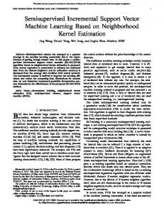
Fig. 1. Left: An exemplary solution of the SVDD. Right: Illustration of SSSVDD that incorporates unlabeled (green) as well as labeled data of the normal class (red) and the rejection category (blue).

4

Semi-supervised Data Domain Description

In this section, we derive our semi-supervised data domain description. In addition to n normal observations x1 , . . . , xn ∈ X we are also given m labeled pairs ∗ ∗ (x∗n+1 , yn+1 ), . . . , (x∗n+m , yn+m ) ⊂ X × {+1, −1}, where we associate normal data with the positive class and outliers as the negative class. As in the previous section, we aim at finding a model f (x) = ||φ(x) − c||2 − R2 that generalizes well on unseen data, however, the model is now devised on the basis of labeled and unlabeled data. A straight-forward extension of the SVDD in Equation (1) using both, labeled and unlabeled examples, is given by min

R,γ,c,ξ

s.t.

2

R − κγ + ηu

n  i=1

ξi + ηl

n+m 

ξj∗

j=n+1

∀ni=1 : φ(xi ) − c2 ≤ R2 + ξi   ∗ ∗ 2 2 ∀n+m j=n+1 : yj φ(xj ) − c − R ∀ni=1 : ξi ≥ 0,

≤ −γ + ξj∗

(2)

∗ ∀n+m j=n+1 : ξj ≥ 0.

The optimization problem has additional constraints for the labeled examples that have to fulfill the margin criterion with margin γ. Trade-off parameters κ, ηu , and ηl balance margin-maximization and the impact of unlabeled and labeled examples, respectively. To avoid cluttering the notation unnecessarily, we omit the obvious generalization of allowing different trade-offs ηl+ and ηl− for positively and negatively labeled instances, respectively. The additional slack variables ξj∗ are bound to labeled examples and allow for point-wise relaxations of margin violations by labeled examples. The solution of the above optimization problem is illustrated in Figure 1 (right). The inclusion of negatively labeled data turns the above optimization problem non-convex and optimization in the dual is prohibitive. As a remedy, we translate

412

N. Görnitz, M. Kloft, and U. Brefeld

Equation (2) into an unconstraint, continuous problem [3,33]. For the above problem, it is possible to resolve the slack terms:   ξi =  R2 − ||φ(xi ) − c||2     ξj∗ =  yj∗ R2 − ||φ(x∗j ) − c||2 − γ where (t) = max{−t, 0} is the common hinge loss where we explicitely deal with the margin γ in the argument t because γ is part of the optimization. We can now pose optimization problem (2) as a simple minimization problem without constraints as follows, min

R,γ,c

R2 − κγ + ηu

n     R2 − ||φ(xi ) − c||2 i=1 n+m 

+ ηl

     yj∗ R2 − ||φ(x∗j ) − c||2 − γ .

(3)

j=n+1

Note that the optimization problems in Equations (2) and (3) are equivalent so far. We now substitute the Huber loss for the hinge loss to obtain a smooth and differentiable function that can be optimized with gradient-based techniques. The Huber loss Δ, is displayed in Figure 2 and given by ⎧ ⎨ Δ−t2 : t ≤ Δ−

Δ, (t) = (Δ+−t) : Δ− ≤t≤Δ+

4 ⎩ 0 : otherwise ⎧ −1 : t≤Δ−

⎨ + 1) : Δ− ≤t≤Δ+

(4) Δ, (t) = − 21 ( Δ−t  ⎩ 0 : otherwise . For notational convenience, we focus on the Huber loss for Δ=0, (t) and move margin dependent terms into the argument t. Using the Huber loss 0, , computing the gradients of the slack variables ξi associated with unlabeled examples with respect to the primal variables R and c yields ∂ξi = 2R (R2 − ||φ(xi ) − c||2 ) ∂R ∂ξi = 2(φ(xi ) − c) (R2 − ||φ(xi ) − c||2 ). ∂c The derivatives of their counterparts ξj∗ for the labeled examples with respect to R, γ, and c are given by     ∂ξj∗ = 2yj∗ R yj∗ R2 − ||φ(x∗j ) − c||2 − γ ∂R     ∂ξj∗ = −κ yj∗ R2 − ||φ(x∗j ) − c||2 − γ ∂γ     ∂ξj∗ = 2yj∗ (φ(x∗j ) − c) yj∗ R2 − ||φ(x∗j ) − c||2 − γ . ∂c

Active and Semi-supervised Data Domain Description

413

1 hinge loss Huber loss

linear

loss

0.75

0.5

quadratic

0.25

linear

0 0

0.5

1 yf(x)

1.5

2

Fig. 2. The differentiable Huber loss δ=1,=0.5

Substituting the partial gradients, we resolve the gradient of Equation 3 with respect to the primal variables: n n+m   ∂ξj∗ ∂ξi ∂EQ3 = 2R + ηu + ηl , ∂R ∂R ∂R i=1 j=n+1

(5)

n+m  ∂ξj∗ ∂EQ3 = −κ + ηl , ∂γ ∂γ j=n+1

(6)

n n+m   ∂ξj∗ ∂EQ3 ∂ξi = ηu + ηl . ∂c ∂c ∂c i=1 j=n+1

(7)

The above equations can be plugged directly into off-the-shelf gradient-based optimization tools to optimize Equation (3) in the input space for the identity φ(x) = x. However, predictive power is often related to (possibly) non-linear mappings φ of the input data into some high-dimensional feature space. An application of the representer theorem (see Appendix) shows that the center c can be expanded as   c= αi φ(xi ) + αj yj∗ φ(x∗j ). (8) i

j

According to the chain rule, the gradient of Equation (3) with respect to the αi/j is given by ∂EQ3 ∂c ∂EQ3 = . ∂αi/j ∂c ∂αi/j Using Equation (8), the partial derivatives ∂c = φ(xi ) ∂αi

and

∂c ∂αi/j

resolve to

∂c = yj∗ φ(x∗j ), ∂αj

(9)

414

N. Görnitz, M. Kloft, and U. Brefeld

respectively. Applying the cain-rule to Equations (5),(6),(7) and (9) gives the gradients of Equation (3) with respect to the αi/j . The final objective function allowing for the use of kernel functions can be stated as min

R,γ,α

R2 −κγ +ηu + ηl

n 

   R2 − k(xi , xi ) + (2ei − α) Kα

i=1 n+m 

     yj∗ R2 − k(x∗j , x∗j ) + (2e∗j − α) Kα − γ , (10)

j=n+1

where kernel K is given by K(x, x ) = φ(x), φ(x ) and e1 , . . . , en+m is the standard base of Rn+m . By rephrasing the problem as an unconstrained optimization problem, its intrinsic complexity has not changed. However, the local minima of Optimization Problems (3) and (10) can now easily be found with gradient-based techniques such as conjugate gradient descent. In general, unconstrained optimization is also easier to implement than constrained optimization. We will observe the benefit of this approach in the following.

5

Active Learning

The SSSVDD is initially trained solely on unlabeled examples and then subsequently refined by incorporating labeled examples that have been queried by the active learning rule. We now devise an active learning strategy to query lowconfidence decisions, hence guiding the user in the labeling process. Our active learning strategy selects an instance of the unlabeled data pool to be labeled by the user. The selection process is designed to find the unlabeled example in the pool which – once labeled – leads to the maximal improvement of the actual model. We begin with a commonly used active learning strategy which simply queries borderline points. The strategy is sometimes called margin strategy and can be expressed by asking the user to label the point x that is closest to the decision hypersphere [1,29] x

=

|f (x)| Ω x∈{x1 ,...,xn } argmin

=

|R2 − φ(x) − c2 | , Ω x∈{x1 ,...,xn } argmin

(11)

where Ω is a normalization constant and given by Ω = maxi |f (xi )|. However, when dealing with many non-stationary outlier and/or attack categories, it is beneficial to identify novel reject classes as soon as possible. We translate this into an active learning strategy as follows. Let A = (aij )i,j=1,...,n+m be an adjacency matrix, for instance obtained by a k-nearest-neighbor approach, where aij = 1 if xi is among the k-nearest neighbors of xj and 0 otherwise. We introduce an extended labeling y¯1 . . . , y¯n+m for all examples by defining y¯i = 0 for unlabeled instances and retaining the labels for labeled instances, i.e.,

Active and Semi-supervised Data Domain Description

415

y¯j = yj . Using these pseudo labels, Equation (12) returns the unlabeled instance according to x

=

n+m 1  (¯ yj + 1) aij . xi ∈{x1 ,...,xn } 2k j=1

argmin

(12)

The above strategy explores unknown regions in feature space and subsequently deepens the learned knowledge by querying clusters of potentially similar objects to allow for good generalizations. Nevertheless, using Equation (12) alone may result in querying points lying close to the center of the hypersphere or far from its boundary. These points will hardly contribute to an improvement of the hypersphere. In other words, only a combination of both strategies (11) and (12) guarantees the active learning to query points of interest. Our final active learning strategy is therefore given by x =

argmin xi ∈{x1 ,...,xn }

=δ

n+m |f (x)| 1 − δ  + (¯ yj + 1) aij Ω 2k j=1

(13)

for δ ∈ [0, 1]. The combined strategy queries instances that are close to the boundary of the hypersphere and lie in potentially anomalous clusters with respect to the k-nearest neighbor graph. Depending on the actual value of δ, the strategy jumps from cluster to cluster and thus helps to identify interesting regions in feature space. For the special case of no labeled points our combined strategy reduces to the margin strategy. Usually, an active learning step is followed by an optimization step of the SSSVDD taking into account the newly labeled data. This procedure is of course time-consuming and can be altered for practical settings, for instance by querying a couple of points before performing a model update. Irrespectively of the actual implementation, alternating between active learning and updating the model can be repeated until a desired predictive performance is obtained.

6

Empirical Results

In this section, we empirically evaluate the SSSVDD and the active learning strategies and compare their performances to appropriate strawmen. The baselines SVDD and SVDDneg [23] are implemented in Matlab and optimized by SMO [18]. Additional baselines for the object recognition tasks are binary SVMs. SSSVDDs are optimized by conjugate gradient descent. Parameters of the active learning strategy are set to k = 10, α = 0.1 for simplicity. We experiment on network intrusion and object recognition tasks. 6.1

Intrusion Detection

For the intrusion detection experiments we use HTTP traffic recorded within 10 days at Fraunhofer Institute FIRST. The data set comprises 145,069 unmodified

416

N. Görnitz, M. Kloft, and U. Brefeld 1

AUC [0,0.01]

0.95 0.9 0.85 0.8 0.75

SSSVDD SVDD SVDDNeg

0.7 0 1 2 3 4 5 7.5 10 labeled data in %

15

Fig. 3. Results for normal vs. malicious

connections of average length of 489 bytes. We refer to the FIRST data as the normal pool. The malicious pool contains 27 real attack classes generated using the Metasploit framework [16]. It covers 15 buffer overflows, 8 code injections and 4 other attacks including HTTP tunnels and cross-site scripting. Every attack is recorded in 2 – 6 different variants using virtual network environments and decoy HTTP servers. To study the robustness of the different approaches in a more realistic scenario we also study techniques to obfuscate malicious content by adapting attack payloads to mimic benign traffic in feature space [6]. As a consequence, the extracted features do not deviate from a model of normality and the classifier is likely to be fooled by the attack. For our purposes it already suffices to study a simple cloaking technique by adding common HTTP headers to the payload while the malicious body of the attack remains unaltered. We apply this technique to the malicious pool and refer to the obfuscated set of attacks as cloaked pool. We focus on two scenarios: normal vs. malicious and normal vs. cloaked data. For both settings, the respective byte streams are translated into a bag-of-3grams representation. For each experiment, we randomly draw 966 training examples from the normal pool and 34 attacks either from the malicious or the cloaked pool, depending on the scenario. Holdout and test sets are also drawn at random and consist of 795 normal connections and 27 attacks, each. We make sure that attacks of the same attack class occur either in the training, or in the test set but not in both. We report on 10 repetitions with distinct training, holdout, and test sets and measure the performance by the area under the ROC curve in the false-positive interval [0, 0.01] (AUC0.01 ) Figure 3 shows the results for normal vs. malicious data pools, where the x-axis depicts the percentage of randomly drawn labeled instances. Irrespectively of the amount of labeled data, the malicious traffic is detected by all methods equally well as the intrinsic nature of the attacks is well captured by the bag-of-3-grams representation. There is no significant difference between the classifiers. However, our next experiment shows the fragility of the of these results in the presence of simple cloaking techniques. Simply obfuscating the attacks by copying normal headers into the malicious payload leads to dramatically different results.

Active and Semi-supervised Data Domain Description 1

0.8

0.7

0.6 01 3 6

SVDD Neg

0.9 AUC [0,0.01]

SVDDNeg SSSVDD

0.9 AUC [0,0.01]

1

SVDD

417

SVDD SSSVDD

0.8

0.7

10

15 22.5 32.5 labeled data in %

47.5

0.6 0 1 2 3 4 5 7.5 10 labeled data in %

15

Fig. 4. Results for normal vs. cloaked. Left: Random samling. Right: Active learning.

Figure 4 (left) displays the results for normal vs. cloaked data. First of all, the performance of the unsupervised SVDD drops to only 70%. We obtain a similar result for the SVDDneg ; incorporating cloaked attack information into the training process of the SVDD leads to an increase of about 5% which is far from any practical value. Notice that the SVDDneg cannot make use of labeled data of the normal class. Thus, its moderate ascent in terms of the number of labeled examples is credited to the class ratio of 966/34 for the random labeling strategy. The bulk of additional information cannot be exploited and has to be left out. By contrast, the semi-supervised SSSVDD includes all labeled data into the training process and clearly outperforms the two baselines. For only 5% labeled data, the SSSVDD easily beats the best baseline and for randomly labeling 30% of the available data it separates almost perfectly between normal and cloaked malicious traffic. Nevertheless, labeling 30% of the data is not realistic for practical applications. We thus explore the benefit of active learning for inquiring label information of borderline and low-confidence points. Figure 4 shows the results for normal vs. cloaked data where the labeled data for SVDDneg and SSSVDD is chosen according to the active learning strategy in Equation (13). The unsupervised SVDD that does not make use of labeled information remains at an AUC0.01 of 70%. Compared to the results for a random labeling strategy (Figure 4, left), the performance of its counterpart SVDDneg increases significantly. The ascent of the SVDDneg is now steeper and yields 85% for 15% labeled data. However, the SSSVDD also improves for active learning and dominates the baselines. Using active learning, we need to label only 3% of the data for attaining an almost perfect separation, compared to 25% for a random labeling strategy. Our active learning strategy effectively boosts the performance and reduces the manual labeling effort significantly. Figure 5 details the impact of our active learning strategy in Equation (13). We compare the number of outliers detected by the combined strategy with the margin-based strategy in Equation (11) (see also [1]) and by randomly drawing instances from the unlabeled pool. As a sanity check, we also included the theoretical outcome for random sampling. The results show that the combined strategy effectively detects malicious traffic much faster than the margin-based strategy.

418

N. Görnitz, M. Kloft, and U. Brefeld 35 30

#outliers

25 20 15 10 5

optimal active learning margin random (empirical) random (theoretical)

0 0 1 2 3 4 5 7.5 10 labeled data in %

15

Fig. 5. Number of outliers found by active learning

6.2

Object Recognition

For our object recognition experiments we use the classification data of the VOC 2008 challenge [5]. The data set comprises 8780 images and 20 object classes. An image is annotated with a class label if at least one object from that class is detectable in the image. We use the training and holdout sets for our experiments which contain 4340 images. For computational reasons, we focus on the three randomly drawn classes aeroplane (198 instances), bird (286 instances), and dog (266 instances), exemplary images are displayed in Figure 6. From the pool, we draw 375 instances randomly as independent test set while the remaining 375 examples are used for model selection over 10 repetitions. In each run, we randomly draw 10 labeled images of each class, 148 unlabeled instances, and 187 holdout examples. We employ pyramid histograms [10] of visual words [4] (PHOW) for pyramid levels 0,1,2 over the grey channel. We obtain a feature vector for every image by concatenating histograms of all levels. For the grey channel, 1200 visual words are computed by k-means clustering on SIFT features [13] from randomly drawn images of each class. The underlying SIFT features are extracted from a dense grid of pitch ten. Figure 7 compares regular support vector machines (SVMs) with SSSVDDs where both approaches apply margin-based active learning (Equation (11)) and the combined strategy in Equation (13) for detecting query points. For only a few labeled data points and many unlabeled examples (which cannot be utilized

Fig. 6. Exemplary images from the VOC2008 object recognition data set. From left to right: aeroplane, dog, and bird.

Active and Semi-supervised Data Domain Description

419

0.5

error

0.4

0.3 SVM combined SVM margin SSSVDD combined SSSVDD margin

0.2

0.1 0

5

10 labeled data in %

25

Fig. 7. Error rates for the VOC2008 data set

by SVMs), both approaches perform comparably. However, for increasing percentages of labeled data, the task becomes more and more a binary problem for which the SVM is well suited. For 25% labeled data, the SVM beats the SSSVDD significantly. Nevertheless, SSSVDD proves robust when labeled data is scarce and expensive to obtain; unlabeled examples are effectively exploited to augment sparse labelings.

7

Conclusion

In this paper, we proposed to view data domain description as a semi-supervised learning problem to allow for the inclusion of prior and expert knowledge. We generalized support vector data description to a semi-supervised learning algorithm (SSSVDD). Since the objective function of the SSSVDD is not convex, we translated the optimization problem into an unconstraint, continuous problem which can be optimized with efficient gradient-based techniques. Furthermore, we proposed a novel active learning strategy to guide the user in the labeling process of the unlabeled data by querying instances that are not only close to the boundary of the hypersphere but also likely members of novel rejection categories. Empirically, we showed on network intrusion detection and object recognition tasks that rephrasing the unsupervised problem setting as a semi-supervised task is worth the effort. For instance in the network intrusion detection task, SSSVDDs prove robust in scenarios where the performance of baseline approaches deteriorate due to obfuscation techniques. Moreover, we observe the effectiveness of our active learning strategy which significantly improves the quality of the SSSVDD and spares practitioners from labeling unnecessarily many data points. Acknowledgements. We thank Konrad Rieck for providing the kernels for the HTTP traffic and Christina Müller and Shinichi Nakajima for helping us with the object recognition task. This work was supported in part by the German Bundesministerium für Bildung und Forschung (BMBF) under the project ReMIND (FKZ 01-IS07007A) and by the FP7-ICT Programme of the European Community, under the PASCAL2 Network of Excellence, ICT-216886.

420

N. Görnitz, M. Kloft, and U. Brefeld

References 1. Almgren, M., Jonsson, E.: Using active learning in intrusion detection. In: Proc. IEEE Computer Security Foundation Workshop (2004) 2. Angiulli, F.: Condensed nearest neighbor data domain description. In: Advances in Intelligent Data Analysis VI (2005) 3. Chapelle, O., Zien, A.: Semi-supervised classification by low density separation. In: Proceedings of the International Workshop on AI and Statistics (2005) 4. Csurka, G., Bray, C., Dance, C., Fan, L.: Visual categorization with bags of keypoints. In: Workshop on Statistical Learning in Computer Vision, ECCV, Prague, Czech Republic, May 2004, pp. 1–22 (2004) 5. Everingham, M., Van Gool, L., Williams, C.K.I., Winn, J., Zisserman, A.: The PASCAL Visual Object Classes Challenge 2008 (VOC2008) Results (2008), http://www.pascal-network.org/challenges/VOC/voc2008/ 6. Fogla, P., Sharif, M., Perdisci, R., Kolesnikov, O., Lee, W.: Polymorphic blending attacks. In: Proceedings of USENIX Security Symposium (2006) 7. Forrest, S., Hofmeyr, S.A., Somayaji, A., Longstaff, T.A.: A sense of self for unix processes. In: Proc. of IEEE Symposium on Security and Privacy, Oakland, CA, USA, pp. 120–128 (1996) 8. Hoi, C.-H., Chan, C.-H., Huang, K., Lyu, M., King, I.: Support vector machines for class representation and discrimination. In: Proceedings of the International Joint Conference on Neural Networks (2003) 9. Knorr, E.M., Ng, R.T.: Algorithms for mining distance-based outliers in large datasets. In: Proceedings of the 24th International Conference on Very Large Data Bases (1998) 10. Lazebnik, S., Schmid, C., Ponce, J.: Beyond bags of features: Spatial pyramid matching for recognizing natural scene categories. In: IEEE Computer Society Conference on Computer Vision and Pattern Recognition, New York, USA, vol. 2, pp. 2169–2178 (2006) 11. Lee, W., Stolfo, S.J.: A framework for constructing features and models for intrusion detection systems. ACM Transactions on Information Systems Security 3, 227–261 (2000) 12. Liu, Y., Zheng, Y.F.: Minimum enclosing and maximum excluding machine for pattern description and discrimination. In: ICPR 2006: Proceedings of the 18th International Conference on Pattern Recognition, Washington, DC, USA, 2006, pp. 129–132. IEEE Computer Society Press, Los Alamitos (2006) 13. Lowe, D.: Distinctive image features from scale invariant keypoints. International Journal of Computer Vision 60(2), 91–110 (2004) 14. Mahoney, M.V., Chan, P.K.: Learning nonstationary models of normal network traffic for detecting novel attacks. In: Proc. of ACM SIGKDD International Conference on Knowledge Discovery and Data Mining (KDD), pp. 376–385 (2002) 15. Mahoney, M.V., Chan, P.K.: Learning rules for anomaly detection of hostile network traffic. In: Proc. of International Conference on Data Mining (ICDM) (2003) 16. Maynor, K., Mookhey, K., Cervini, J.F.R., Beaver, K.: Metasploit toolkit. Syngress (2007) 17. Pelleg, D., Moore, A.: Active learning for anomaly and rare-category detection. In: Proc. Advances in Neural Information Processing Systems (2004) 18. Platt, J.C.: Fast training of support vector machines using sequential minimal optimization. In: Advances in kernel methods: support vector learning (1999)

Active and Semi-supervised Data Domain Description

421

19. Rieck, K., Laskov, P.: Detecting unknown network attacks using language models. In: Büschkes, R., Laskov, P. (eds.) DIMVA 2006. LNCS, vol. 4064, pp. 74–90. Springer, Heidelberg (2006) 20. Rieck, K., Laskov, P.: Language models for detection of unknown attacks in network traffic. Journal in Computer Virology 2(4), 243–256 (2007) 21. Schölkopf, B., Smola, A.J.: Learning with Kernels. MIT Press, Cambridge (2002) 22. Stokes, J.W., Platt, J.C.: Aladin: Active learning of anomalies to detect intrusion. Technical report, Microsoft Research (2008) 23. Tax, D.M.J.: One-class classification. PhD thesis, Technical University Delft (2001) 24. Tax, D.M.J., Duin, R.P.W.: Support vector data description. Machine Learning 54, 45–66 (2004) 25. Thottan, M., Ji, C.: Anomaly detection in ip networks. IEEE Transactions on Signal Processing 51(8), 2191–2204 (2003) 26. Wang, J., Neskovic, P., Cooper, L.N.: Pattern classification via single spheres. In: Computer Science: Discovery Science, DS (2005) 27. Wang, K., Parekh, J.J., Stolfo, S.J.: Anagram: A content anomaly detector resistant to mimicry attack. In: Zamboni, D., Krügel, C. (eds.) RAID 2006. LNCS, vol. 4219, pp. 226–248. Springer, Heidelberg (2006) 28. Wang, K., Stolfo, S.J.: Anomalous payload-based network intrusion detection. In: Jonsson, E., Valdes, A., Almgren, M. (eds.) RAID 2004. LNCS, vol. 3224, pp. 203–222. Springer, Heidelberg (2004) 29. Warmuth, M.K., Liao, J., Rätsch, G., Mathieson, M., Putta, S., Lemmen, C.: Active learning with support vector machines in the drug discovery process. Journal of Chemical Information and Computer Sciences 43(2), 667–673 (2003) 30. yan Yeung, D., Chow, C.: Parzen-window network intrusion detectors. In: Proceedings of the Sixteenth International Conference on Pattern Recognition, pp. 385–388 (2002) 31. Yuan, C., Casasent, D.: Pseudo relevance feedback with biased support vector machine. In: Proceedings of the International Joint Conference on Neural Networks (2004) 32. Zhu, X.: Semi–supervised learning in literature survey. Technical Report 1530, Computer Sciences, University of Wisconsin-Madison (2005) 33. Zien, A., Brefeld, U., Scheffer, T.: Transductive support vector machines for structured variables. In: Proceedings of the International Conference on Machine Learning (2007)

422

N. Görnitz, M. Kloft, and U. Brefeld

Appendix In this section, we show the applicability of the representer theorem for semisupervised support vector domain descriptions. Theorem 1 (Representer Theorem [21]). Let H be a reproducing kernel Hilbert space with a kernel k : X × X → R, a symmetric positive semi-definite function on the compact domain. For any function L : Rn → R, any nondecreasing function Ω : R → R. If   J ∗ := min J(f )f ∈H := min f ∈ H{Ω ||f ||2H + L (f (x1 ), . . . , f (xn ))} is well-defined, then there exist α1 , . . . , αn ∈ R, such that f (·) =

n 

αi k(xi , ·)

(14)

i=1

achieves J(f ) = J ∗ . Furthermore, if Ω is increasing, then each minimizer of J(f ) can be expressed in the form of Eq. (14). Lemma 1. The representer theorem can be applied to Equation (3). Proof. Recall the primal SSSVDD objective function which is given by J(R, γ, c) =R2 − κγ + ηu

n     R2 − ||φ(xi ) − c||2 i=1

n+m 

+ ηl

     yj∗ R2 − ||φ(x∗j ) − c||2 − γ .

j=n+1

Substituting T := R2 − ||c||2 leads to the new objective function J(T, γ, c) =||c||2 + T − κγ + ηu

n     T − ||φ(xi )||2 + 2φ(xi ) c i=1

+ ηl

n+m 

     yj∗ T − ||φ(x∗j )||2 + 2φ(x∗j ) c − γ .

j=n+1

Expanding the center c in terms of labeled and unlabeled input examples is now covered by the representer theorem. After the optimization, T can be easily resubstituted to obtain the primal variables R, γ, and c.