Active Learning for Data-Driven Verification of ...

Active Sampling for Constrained Simulation-based Verification of Uncertain Nonlinear Systems

arXiv:1705.01471v1 [cs.SY] 3 May 2017

John F. Quindlen1

Ufuk Topcu2

Abstract— Increasingly demanding performance requirements for dynamical systems necessitates the adoption of nonlinear and adaptive control techniques. While satisfaction of the requirements motivates the use of nonlinear control design methods in the first place, the nonlinearity of the resulting closed-loop system often complicates verification that the system does indeed satisfy the requirements at all possible conditions. Current techniques mostly rely upon analytical function-based approaches to certify satisfaction of the requirements. However, for many complex nonlinear systems, it is difficult to find a suitable function with minimally-conservative results to provably certify the system’s response, if one can be found at all. This work presents data-driven procedures for simulation-based, statistical verification in place of analytical proofs. The use of simulations also enables the computation of an approximate solution within a set time or computational threshold, which is not possible with analytical techniques. Active sampling algorithms are developed to iteratively select additional training points to maximize the accuracy of the predictions while constrained by a sample budget. In particular, sequential and batch active sampling procedures using a new binary classification entropy-based selection metric are developed. These approaches demonstrate up to 40% improvement over existing approaches when applied to two case studies in control systems.

I. I NTRODUCTION In high performance systems such as aircraft, the system is expected to satisfy numerous criteria in order for that system to be considered “safe” or “satisfactory”. For example, not only does an aircraft need to be stable, but the aircraft design must also meet handling, maneuvering, and emergency requirements [1], [2]. In such applications, control systems are implemented to help satisfy these criteria under various uncertainties by controlling the closed-loop trajectory response. Verification procedures can then be used to ensure the resulting closed-loop system does in fact satisfy the requirements under all possible conditions. As the demand for higher performance and/or efficiency grows, more advanced nonlinear control techniques will be relied upon to achieve the increasingly-complex requirements associated with such demands. While methods such as model reference adaptive control (MRAC) [3] and reinforcement learning (RL) [4] have demonstrated large improvements in performance and efficiency, the challenge with complex control techniques is certifying that the closed-loop system can 1 Graduate Student, Department of Aeronautics and Astronautics, Massachusetts Institute of Technology 2 Assistant Professor, Department of Aerospace Engineering and Engineering Mechanics, University of Texas at Austin 3 Assistant Professor, Departments of Agricultural & Biological Engineering and Aerospace Engineering, University of Illinois Urbana-Champaign 4 Richard C. Maclaurin Professor of Aeronautics and Astronautics, Aerospace Controls Laboratory (Director), MIT

Girish Chowdhary3

Jonathan P. How4

actually meet the requirements for all possible uncertainties. This is due to the nonlinear (and possibly adaptive) nature of the controller, which may result in drastically different trajectories given only slightly different operating conditions. This is exacerbated by any nonlinearities in the open-loop plant itself. Various verification techniques attempt to address this certification problem. If closed-form difference or differential equations of the closed-loop system are known or can be formed, then it may be possible to construct analytical certificates [5]–[7]. These certificates the basis for proofs that provably verify the closed-loop system satisfies the necessary requirements. While such proofs are extremely useful, they are difficult to implement of many systems of interest. For one, closed-form equations of the system may not be known or feasible. Simulation-guided analytical methods [7]–[9] have been developed to help address this, but are limited to certain dynamics. Even if a proof can be constructed, the results may be overly conservative due to the reliance upon specific analytical functions for construction of the proof [10]. Thus, existing analytical verification techniques are not able to suitably certify the satisfaction of the requirements in many nonlinear systems. Data-driven methods [11] are an alternative to analytical verification techniques to address their limitations for such systems. In particular, simulations of the closed-loop system can be used to construct statistical certificates of safety. While statistical certificates are less absolute than analytical proofs, they do not suffer from the same limitations as the previous proof-based techniques and apply to a wider range of systems. In fact, data-driven verification techniques can be used on any virtually system with a suitable simulation model of the dynamics. A suitable simulation model could include everything up to the highest-fidelity imitations of reality such as a full-motion flight training simulator. While statistical certificates produced by data-driven verification are able to produce a solution to a wider range of systems, the accuracy of the certificate is restricted by the quality of the simulation data. If the observed simulation data fails to adequately cover the entire space of possible perturbing uncertainties, then the accuracy of the statistical certificate’s predictions in those unobserved regions will be limited. Conversely, while one solution is to obtain a large, highly-discretized set of simulations spanning the space, simulations can be expensive to obtain. High-fidelity simulation models of the system may be computationally intensive and can form a bottleneck during the verification process. Therefore, it best to carefully select simulations so

as to minimize utilization of the model while maximizing the accuracy of the predictions. In many applications, verification is only part of a higherlevel process such as robust nonlinear control policy design or optimization. In those cases, verification is used to test the suitability of a candidate control policy over the set of given uncertainties. The extra challenge with that is the verification procedure should be able to return a robustness estimate within a reasonable amount of time or effort because the procedure will have to repeated for every candidate control policy. Data-driven methods are particularly suited to this application as they can produce a solution within a set limit by bounding the number of simulations. While this cap will have implications on the accuracy of the robustness estimate, analytical proof-based techniques simply can not guarantee those restrictions will be met. The expected cap on the number of simulations also reinforces the need for careful selection of simulations to maximize accuracy of the predictions. This work addresses those restrictions on the number of simulations with active learning-based sampling procedures. Active sampling [12] methods are closed-loop procedures that iteratively construct a model and then select new training locations to most improve that model. In particular, signal temporal logic [13]–[15] (STL) is used to measure satisfaction of the performance requirements during the simulation trajectories. These measurements are then used to train Gaussian process [16] (GP) regression models that predict the satisfaction of the requirements at unseen perturbations. Existing active learning selection metrics [12], [17] are not ideally suited to this verification problem. Binary support vector machine (SVM) approaches [17] fail to take advantage of the availability of real-valued STL measurements while variance reduction-based sampling criteria [12], [18] ignore the binary nature of predictions: requirements are either satisfied or they’re not. Instead, new tailor-made selection metrics based on binary classification entropy are introduced. Binary classification entropy captures the binary nature of the procedure and can be readily computed using the GP regression model. This new selection metric can then be incorporated into sequential and batch (multiple samples at once) active sampling procedures to select future training locations to improve the predictions. The paper is structured as follows. Section II introduces the problem and describes STL methods for measuring satisfaction of the system requirements from simulation trajectories. Section III then discusses how these measurements can be used to construct a Gaussian process prediction model and estimate the confidence in those predictions. Closed-loop active sampling procedures that iteratively select training locations to improve the GP prediction model are shown in Section IV. Given a budget on the number of samples, these procedures will attempt to form the best training set to produce the most accuracy statistical certificate. Finally, Section V demonstrates these processes on two example problems: a model reference adaptive controller and an aircraft autopilot. Both of these case studies have uncertain

nonlinear dynamics that are exceedingly difficult to analyze using proof-based techniques. The results will also show the entropy-based active sampling procedures outperform existing approaches for verification problems. II. P ROBLEM F ORMULATION Consider the following nonlinear system x(t) ˙ = f (x(t), u(t), θ)

(1)

where x(t) ∈ Rn is the state vector and u(t) ∈ Rm is the control input vector. In this work, an exact simulation model of f (x(t), u(t), θ) is assumed to be known and available for verification. The system is also perturbed by parametric uncertainties θ ∈ Rp that affect the state dynamics. While the exact values of θ at run-time are unknown during the time of verification, their effects in f (x(t), u(t), θ) and the set of all feasible perturbations θ ∈ Θ are assumed to be known. For example, θ could include initial conditions x(0) and mass/inertia properties of a physical system. Lastly, as the emphasis is on verification of the closed-loop system, the control policy u(t) = g(x(t)) is assumed to be known. Let the trajectory of the closed-loop system in the time interval t ∈ [0, Tf ] be given by Φ(x(t)|x0 , θ). The trajectory Φ(x(t)|x0 , θ) can be completely determined from x0 and θ. Here, x0 is a fixed nominal initial condition. If the true initial condition x(0) is uncertain (x(0) 6= x0 ), then x(0) can still be modeled as the combination of the known nominal initial condition x0 and the unknown perturbations, i.e. x(0) = x0 +θ. The resulting trajectory Φ(x(t)|x0 , θi ) will ultimately determine whether the performance requirements were satisfied at a particular θi perturbation. A. Requirement Modeling The closed-loop system trajectory is expected to satisfy certain performance criteria, assumed to be given a-priori. These criteria may be given by a wide variety of sources and can include relatively straightforward concepts like stability or boundedness as well as more complex spatio-temporal requirements such as those specified in civil or military aviation regulations [1], [2]. In order to capture the wide range of possible specifications, the performance requirements are modeled using temporal logic specifications. In particular, these specifications are given by signal temporal logic (STL). Signal temporal logic provides a mathematical language for expressing the requirements and measuring their satisfaction in Φ(x(t)|x0 , θ). The following subsection will briefly overview STL and its applications to the problem. More formal, comprehensive descriptions of STL are found in [13]–[15]. A requirement of interest is given as a STL formula ϕ. This formula consists of predicates ζ that are functions of the state (and possibly control input) values and Boolean and temporal operations on those predicates. The predicate ζ defines inequalities for functions of the state, input values such that ζ > 0. For example, if state x1 (t) must remain above 2, then the corresponding predicate isζ = x1 (t) − 2 > 0. Temporal operators include [t1 ,t2 ] , ♦[t1 ,t2 ] , and U[t1 ,t2 ] ,

which express that a predicate must hold “always”, “at some time”, and “until another predicate” between between times t1 and t2 . Meanwhile, the Boolean operators ¬, ∧, and ∨ can be used alongside the temporal operators to express negation, conjunction, and disjunction. Tuple (Φ, t) |= ϕ then signifies that trajectory Φ satisfies requirement formula ϕ at time t and (Φ, t) |= ¬ϕ signifies failure. More complex formulas can be constructed from combinations of these operators and simpler formulas. For example, consider formula ϕ3 = [t1 ,t2 ] ϕ1 ∧♦[t2 ,t3 ] ϕ2 , which states ϕ1 must hold for all times between t1 and t2 and ϕ2 must occur at some point between t2 and t3 . In a similar fashion, the conjunction operator can also be used when multiple requirements, say i = 1 : N , must be considered simultaneously in order to construct one VN large formula, i.e. ϕ = i=1 ϕi . One difference of STL over other temporal logic representations is the inclusion of a real-valued robustness degree ρϕ ∈ R. This robustness degree not only classifies whether the trajectory satisfied the requirement ϕ, but also quantifies how well it satisfied the requirement or how badly it failed to meet it. Essentially, ρϕ > 0 signifies satisfaction of ϕ while ρϕ ≤ 0 signifies failures to satisfy ϕ. Remark 1 Note that ρϕ = 0 is slightly ambiguous and is assumed to represent failure to meet ϕ, as in [15]; however, ρϕ = 0 has been deemed satisfactory in other works [14]. A more detailed description of the robustness degree is found in [13], but a short summary of the terms used in this paper are included below, taken from [14]: ρϕ (t) = ζ(t) ρ[t1 ,t2 ] ϕ (t) = ρ

♦[t1 ,t2 ] ϕ

(t) =

min

t0 ∈[t+t1 ,t+t2 ]

max

t0 ∈[t+t1 ,t+t2 ] ϕ1

0

ρ (t )

Assumption 1 There exists a sufficiently fine discretization of Θ, Θd , at whose θ values simulations can be performed. In order for the discretization Θd to suitably capture the potential non-convexity of Θs and Θf , the size |Θd | will be large. Even with this discretization of Θ, it will be infeasible to perform simulations at every θ ∈ Θd . To model this effect, the verification procedure is assumed to be constrained by a computational budget. Assumption 2 The simulation-based verification procedure is constrained by a computational budget. This computational budget is assumed to manifest as a cap on the number of simulations, Ntotal , allocated to the verification procedure. This assumption constraining the number of simulations allocated to the verification is motivated by the work in [19] where a simulator of forest fire dynamics required a large amount of computational resources for the simulation of a single fire trajectory (roughly 1-3 minutes per trajectory on a desktop computer). It would be impractical to run a large number of simulations at every possible condition, especially when a predicted would need to be computed within a reasonable time window (1-2 hours) in realistic scenarios. III. S IMULATION - BASED P REDICTIONS

ρϕ (t0 ) ϕ

In many applications, the system in Eq. 1 is too complex to suitably analyze and verify with any other method than through simulation rollouts. In that case, simulation trajectories are used to observe ρϕ (θ) and estimate Θs and Θf .

(2)

ρϕ1 ∧ϕ2 (t) = min (ρ (t), ρϕ2 (t)). The term ρϕ (t) refers to the robustness degree measured at time t and ρϕ (t) > 0 indicates that ϕ is satisfied for all times starting from time t. In this paper, the entire trajectory from t = 0 to t = Tf is considered; therefore, ρϕ (t = 0) is used to verify the entire trajectory Φ satisfies the requirements. For simplicity, the time indices will be dropped for the remainder of this paper, i.e. ρϕ = ρϕ (t = 0). Remark 2 The trajectory Φ(x(t)|x0 , θ) will change according to θ, which will in turn affect the satisfaction of ϕ and its correspond robustness degree ρϕ . To emphasize this fact, the robustness degree will be subsequently written as ρϕ (θ). B. Problem Description Problem 1 The goal of the verification procedure is to separate Θ into the set of all θ values for which ρϕ (θ) > 0, Θs , and the set of all perturbations for which ρϕ (θ) ≤ 0, Θf . By definition, Θs ∪ Θf = Θ and Θs ∩ Θf = ∅.

With the constraints from Assumption 2, the problem now becomes the construction of an accurate approximation of Θs and Θf from Problem 1 while limited to Ntotal simulation trajectories. Previous work in simulation-based proof techniques bridged the gap between analytical proof techniques and pure data-driven methods; however, these approaches were either unable to produce an accurate estimate of Θs /Θf [10] or failed to guarantee an answer could be produced at all. Instead, this work focuses entirely on the data-driven approach. A regression model can be constructed from observed simulation trajectories and ρϕ (θ) in order to predict ρϕ (θ) at all other θ ∈ Θd and estimate whether the trajectories will satisfy ϕ or not. A. Gaussian Process Regression Model A Gaussian process (GP) regression model can be constructed from a training dataset L of initial observations. This training dataset consists of N pairs of θ values and their measured ρϕ (θ) robustness degrees. The set of N observed θ locations is vector θL = [θ1 , θ2 , . . . θN ]T while the ρϕ (θ) are grouped in vector yL = [ρϕ (θ1 ), ρϕ (θ2 ), . . . ρϕ (θN )]T . The training dataset is then L = {θL , yL }. Gaussian processes have been used extensively to create Bayesian nonparametric models of unknown functions using a finite collection of training data. In short, a GP defines

a distribution over possible functions that can be used to predict the response over unobserved regions of Θ. A more in-depth discussion of GPs is found in [16]. The end result of the training process is a posterior predictive mean µ(θ) and covariance Σ(θ) to estimate ρϕ (θ), where the estimated ρbϕ (θ) is ρbϕ (θ) ∼ N (µ(θ), Σ(θ)). The posterior mean and covariance are computed by µ(θ) = κ(θ, θL ) κ(θL , θL )−1 yL Σ(θ) = κ(θ, θ) − κ(θ, θL ) κ(θL , θL )−1 κ(θL , θ),

(3)

where κ(θ, θL ) is a 1 × N vector of κ(θ, θi ) ∀i = 1 : N and κ(θL , θL ) is a N × N matrix of κ(θi , θj ) ∀i, j = 1 : N . The term κ(., .) refers to the kernel function, of which there are many possible candidates. This paper uses the squared exponential kernel with automatic relevance determination (ARD) κ(θ, θ0 ) = σf2 exp{−0.5(θ − θ0 )T D−1 (θ − θ0 )}

(4)

D = diag(σ12 , σ22 , . . . , σp2 ). The kernel hyperparameters are σ = {σf , σ1 , σ2 , . . . σp }. In comparison to the isotropic squared exponential kernel with σ1 = σ2 = . . . = σp , the ARD kernel enables the hyperparameters to vary and thus deemphasize θ components with minimal impact upon ρϕ (θ) or emphasize those with high sensitivity. Remark 3 The Gaussian process regression model in Eq. 3 is a noise-free GP [16]. Most Gaussian process models use a homoscedastic Gaussian noise term to model measurement noise in the observations. That assumption does not apply in this application with deterministic simulations of the trajectory and ρϕ (θ) measurements taken directly from Φ(x(t)|x0 , θ). Upcoming work by the authors will address the problem of stochastic simulations. B. Prediction Confidence While the GP regression model predicts the real-valued robustness degree, the verification problem is fundamentally a binary classification problem: concerned with whether ρϕ (θ) > 0 or ρϕ (θ) ≤ 0, rather than the exact value of ρϕ (θ) itself. This highlights the fact that not all predictions are weighted equally. Higher estimation error is acceptable further away from the boundary ρϕ (θ) = 0 than nearby. The predicted satisfaction, z(θ|L) = {1, −1}, corresponding to ρϕ (θ) > 0 and ρϕ (θ) ≤ 0 is fairly straightforward: z(θ|L) = sign µ(θ)

(5)

and z(θ|L) = −1 at µ(θ) = 0. The use of STL with real-valued robustness degrees rather than binary measurements such as those used by Metric temporal logic also enables the confidence in the predictions from Eq. 5 to be quantified. Earlier work in data-driven verification [11] focused entirely on binary measures of satisfaction which effectively indicated only the sign of ρϕ (θ).

Now with the real-valued measurements, the probability of satisfaction at each θ location can be computed through a Gaussian cumulative distribution function (CDF) using µ(θ) and Σ(θ) 1 1  µ(θ)  . P(ρϕ (θ) > 0|L, σ) = P+ (θ|L, σ) = + erf p 2 2 2Σ(θ) (6) It is important to note that this probability of satisfaction is dependent upon the training data L and the corresponding GP mean µ(θ) and covariance Σ(θ) functions. Changes to the latter two will affect the distribution and thus affect the computed probability. The following subsection will discuss the importance of the hyperparameters used to construct µ(θ) and Σ(θ) and their effect on the prediction confidence. C. Hyperparameter Optimization The choice in hyperparameters σ greatly affects the GP regression model and the resulting posterior predictive distribution ρbϕ (θ) ∼ N (µ(θ), Σ(θ)). In the vast majority of related works [18], [20]–[22], there is little-to-no mention of the choice of hyperparameters. In some works [21], the convergence guarantees of the algorithms presented are dependent upon the fact the ideal (true) choice of hyperparameters is known apriori and fixed. In practice, this assumption cannot be made as little is known about the distribution of the robustness degree over Θ until after simulations are performed. Instead, the hyperparameters must be chosen with only the current available information, training dataset L. The distribution of the hyperparameters with respect to the training set L is given by P(σ|yL , θL ) = R

P(yL |θL , σ)P(σ) . P(yL |θL , σ)P(σ)dσ

(7)

Without prior information about the choice of σ, the distribution P(σ) can be assumed to be uniform. The issue with Eq. 7 is that there is no closed-form solution to compute P(σ|yL , θL ) so sampling-based approximation or Markov Chain Monte Carlo (MCMC) methods must be used to construct the probability distribution [16]. However, such approaches are intractable for the resource-constrained problem considered here; every sample from P(yL |θL ) requires the inversion of the N × N matrix κ(θL , θL ), an O(N 3 ) operation. Instead, hyperparameter optimization can be used to approximate the maximum likelihood estimate (MLE) of the hyperparameters. From Eq. 7, the hyperparameter distribution P(σ|θL , yL ) is proportional to P(yL |θL ); therefore, the MLE of P(yL |θL ) will also correspond to the MLE of σ. A local maximum to P(yL |θL ) can be computed using steepest descent methods as in [16] or gradient-based methods from [23]. As mentioned earlier, the ARD squared exponential kernel enables less-influential θ components to be deemphasized. When little is known about the hyperparameters apriori, this optimization procedure is particularly useful for discovering these less-influential components from the observed data L and subsequently adjusting the sensitivity. Even though the optimization framework can only guarantee local optimums,

the results in Figure 6 of Section V indicate hyperparameter optimization will provide improved prediction error over static hyperparameters. The choice in hyperparameters will also affect the CDF from Eq. 6 describing the probability of satisfaction of ϕ. If the true hyperparameters, labeled σ ∗ , are known, then the actual probability P(ρϕ (θ) > 0|L) = P(ρϕ (θ) > 0|L, σ ∗ ); however, this is a very restrictive assumption. In the more likely case when the true hyperparameters σ ∗ are not known, the the probability of satisfaction is the marginal likelihood over all possible σ Z P(ρϕ (θ) > 0|L) = P(ρϕ (θ) > 0|L, σ)P(σ|yL , θL )dσ. (8) Since this integral requires P(σ|yL , θL ), the computation of the total probability in Eq. 8 is intractable as well. Since there is no closed-form solution, the same approximation or sampling methods must be used. All the effort used to approximate P(σ|yL , θL ) could be used to obtain additional simulations. IV. ACTIVE S AMPLING Given a set of training data, a data-driven statistical model can be constructed to provide predictions over the entire Θ space; however, these predictions are highly dependent upon the training dataset L. With L limited to Ntotal samples, it is crucial that the best possible set is chosen, especially when Ntotal is small compared to |Θd |. As would be expected, the difficulty lies in the fact that the ideal training set is unknown ahead of time. Rather than passively select training datapoints, either randomly or in a structured grid, training samples can be actively chosen in a closed-loop fashion. Active learning procedures [12] include a variety of different approaches, all of which attempt to identify the “best” samples to obtain in order to improve a statistical model. Depending on the application and objectives, the definition of the “best” sample will change, even for the same exact model. One of the most general approaches is the expected model change (EMC)/uncertainty sampling metric [17]. Though widely-applied to support vector machine (SVM)-based models, EMC also applies to Gaussian process regression models. The underlying selection metric for the “best” sample θ is the point most likely to induce the largest expect change in the model; in short, this means θ = argmin |µ(θ)|. Another approach is variance reduction [12], [18]. While various approximations or derivations exist [18], the end goal is to select θ which most reduces the posterior variance of the GP model. Since it is comparatively expensive, although possible, to calculate the change in posterior variance, the most common approximation is to select θ = argmax Σ(θ). Regardless of the efficiency or accuracy of the approaches or their approximations, none of these approaches directly address the underlying objective in this verification problem: to predict whether ρϕ (θ) > 0 or not. Instead of the other selection metrics, binary classification entropy is used to identify informative sample locations.

Unlike variance methods, which may also use the term “entropy” [18], binary classification entropy considers the probability P(ρϕ (θ) > 0) from Eq. 6 rather than the entropy of Σ(θ). The binary classification entropy at a location θ for a given (L, σ) is  H(θ|L, σ) = − P+ (θ|L, σ)log2 P+ (θ|L, σ) (9)  + (1 − P+ (θ|L, σ))log2 (1 − P+ (θ|L, σ)) . The total entropy over Θd can be determined by summing Eq. 9 over all unobserved θ locations (entropy ∀θ ∈ L is 0). This set of unobserved sample locations is listed as U = Θd \ θ L |U | X H(U|L, σ) = H(θi |L, σ). (10) i=1

A. Sequential Sampling Ideally, the best sample location θ would induce the largest possible change in total entropy (Eq. 10), !     θ = argmax H U|L ∪ {θ0 , y(θ0 )}, σ − H U|L, σ . θ 0 ∈U

(11) While it is possible, albeit computationally expensive, to compute the posterior reduction in variance, it is actually impossible to compute the posterior classification entropy  H U|L ∪ {θ0 , y(θ0 )}, σ in Eq. 11. The computation of the total posterior classification entropy requires the mean function µ(θ) in order to determine the corresponding P(ρϕ (θ) > 0|L ∪ {θ0 , y(θ0 )}, σ). Since the posterior predictive mean requires the ρϕ (θ) measurement at each training location, the measurement ρϕ (θ) would have to be known in order to compute the entropy. If this measurement were already known, then there would be no need to choose that location as a future sample. Note that variance-focused methods are able to compute the posterior reduction in the variance, albeit expensively, precisely because variance Σ(θ) is independent of the actual measurements and only depends on the measurement locations. In place of the infeasible selection criteria proposed in Eq. 11, a new selection metric is given below: !  θ = argmax H(θ0 |L ∪ {θ0 , y(θ0 )}, σ − H(θ0 |L, σ) θ 0 ∈U

= argmin H(θ0 |L, σ).

(12)

θ 0 ∈U

In this metric, only the current measurements are used, thus avoiding the problem from before. This approach selects the sample location from U with the largest magnitude of classification entropy because it will have the largest change in local entropy. Once a sample is taken, the entropy at that location is 0; therefore, the point with the largest magnitude of classification entropy would have the largest change. Note that the binary classification entropy is strictly non-positive.

A closed-loop sampling procedure using the selection metric from Eq. 12 is listed in Alg. 1. As the process must first start with an initial model in order to compute H(θ|L, σ), the algorithm assumes a GP model has been trained from some initial training set L. Assuming this initial training set counts against the sampling budget Ntotal , there are T additional samples that can be selected, where T = Ntotal − |L|. With the initial GP model, the algorithm first computes the binary classification entropy (Step 3). Steps 4-8 select the “best” sample θ, obtain the measurement at that location, update L and U and retrain the GP model. As part of the retraining process in Step 8, the hyperparameters are re-optimized to reflect the new L with the new sample. This process in Steps 3-8 is repeated until the sampling budget is filled. Algorithm 1 Sequential active sampling algorithm 1: 2: 3: 4: 5: 6: 7: 8: 9:

Input: training set L, available sample locations U, # of additional samples T , trained regression model GP for i = 1 : T do Compute entropy H(θ|L, σ) ∀θ ∈ U Select sample θ from U according to Eq. 12 Run simulation, obtain measurement y(θ) L ← L ∪ {θ, y(θ)} U ← U \ {θ} Retrain regression model GP with new L end for

B. Batch Sampling While the sequential sampling procedure in Alg. 1 will correctly guide the selection of sample points as intended, it requires a large amount of computational effort to continuously recompute the GP after each iteration. Due to the matrix inversion, the cost of each retraining step in Step 8 is O(|L|3 ) or O(|L|2 ) at best, and some multiple of O(|L|3 ) when hyperparameter optimization is performed. Additionally, the cost of predicting the satisfaction of ϕ and computing the entropy at all prospective sampling locations θ ∈ U is O(|L|2 |U|). While Assumption 2 assumes that the primary source of computational cost is the simulation trajectories, the cost associated with each training and prediction step is non-negligible and grows with |L|. Thus, it is also best to minimize the number of retraining steps as much as possible without sacrificing accuracy. One of the most practical methods for reducing the retraining cost is to obtain samples in batch - select multiple θ samples in between retraining steps. Batch active sampling methods [12], [17], [21], [22] are a common tool to lower the training cost and can also inherently take advantage of any parallel computing capabilities to compute multiple simulation trajectories in parallel. In these approaches, M datapoints are chosen at once and their corresponding trajectories are performed in parallel. The challenge with such approaches is ensuring adequate diversity in the chosen set of θ locations to avoid the repeated selection of the same point.

1) Batch Version of Algorithm 1: A straightforward conversion of Algorithm 1 into a batch procedure is shown in Algorithm 4 in Appendix VII-A. As part of the procedure in Alg. 4, the remaining budget allocated to simulations after the initial training set is assumed to be broken evenly into T batches of M points each, for T ×M = Ntotal − |L|. A detailed discussion of the procedure is found in the appendix. As touched upon in that discussion, there are two main issues with the procedure in Alg. 4. First, it is impossible to correctly measure the effects of points previously selected in the batch when choosing the remaining points of the batch. The sample locations previous selected for the batch are stored in a temporary set S. One way to encourage diversity is to update the entropy H(θ|L, σ) to reflect the change in P+ (θ|L, σ) caused by the preceding points in S. While it is possible to compute the change in Σ(θ) without the corresponding measurements yS , it is impossible to update µ(θ) without those. Algorithm 4 approximates the change in entropy by updating Σ(θ) with each additional point in S but freezes the mean µ(θ) to the values from the start of the batch. However, this scales poorly with M since the approximate entropy further diverges from the true entropy with every additional point in S. The second problem with Alg 4 is the high computational load. Because Σ(θ) is updated and the entropy is recomputed ∀θ ∈ U (Step 7 in Alg. 4), each additional point in S requires O(|L∪S|2 )+O(|L∪S|2 |U|) operations, assuming best-case matrix inversion and hyperparameters σ are fixed during the batch. Upon completion of the batch, the hyperparameters will have to be re-optimized with the new training dataset L ← L ∪ {S, yS } and incur the same O(|L|3 ) + O(|L|2 |U|) cost as before in Step 8 of Alg 1. While this approach still ultimately allows for parallel simulations to be performed and introduces the same computational savings associated with those, the cost of selecting the θ perturbations for those simulations is non-negligible. 2) Related Work: Just as there are multiple sequential sampling selection metrics, numerous batch sampling methods have been proposed, usually as a derivate of the aforementioned sequential procedures. Batch EMC algorithms [12], [17] incorporate a diversity measure based upon temporary RBF kernels placed at each θ ∈ S to penalize points in close proximity to θ ∈ S. Batch variance methods are mostly unchanged from their sequential versions [12], [18]. As discussed in the proceeding paragraphs, the covariance function can be updated for S without requiring the corresponding measurements. Therefore, the change in variance is explicitly known before the simulations are even performed and the selection metric need not be modified. The closest prior work is the sampling procedure in [21]. Gaussian process regression models are used to identify level sets and active learning identifies future training points to improve level set estimation. The approach uses the mean function along with confidence intervals based upon the covariance function to predict level sets. The procedure addresses a variant of batch processes not considered by this paper: measurements of selected samples are delayed

by a set number of iterations, much like a time delay. While not perfectly suited to the problem here, the approach does face similar issues with selection of training points before measurements are available at all previously selected sample locations. It was shown that the information gain can be bounded by a fixed quantity and used to bound the change in confidence intervals even without measurements at the “time-delayed” sample locations. Unfortunately, this bound on the information gain is not appropriate to the verification problem considered in this work. First, the bound on information gain strictly assumes the ideal hyperparameters are known and thus the hyperparameters are static and not updated. Additionally, the information bound is inversely proportional to the square the measurement noise. For problems were there is littleto-no measurement noise, as is the case for deterministic simulations of Eq. 1, the bound on the information gain is infinite and of no use. Lastly, the procedure requires updates to the covariance function at each iteration, much like Alg. 4 and batch-variance methods, and therefore suffers from the same heavy computational overhead. 3) Importance Weighting: Rather than rely upon the expensive and flawed batch approximation of the sequential sampling algorithm (Alg. 4), two parallel approaches for batch active sampling are introduced. Both of these approaches utilize importance weighting, essentially importance sampling [24] without the subsequent probability estimate, to efficiently select samples using only the current entropy. Unlike the other batch procedures that update the covariance function after the selection of each point in S, these two approaches freeze the information and select the entire batch of M samples without any intermediate retraining. The crux of the procedures is importance-weighted random sampling: samples for S are randomly chosen based upon some probability distribution. Here, the current entropy H(θ|L, σ) is used to construct the probability distribution from which samples are chosen, where regions with a large magnitude of entropy will have a higher probability of selection. The more straightforward of the two approaches is the baseline importance-weighted sampling procedure shown in Alg. 2. Given some initial training set L and an initial GP model trained from this L, the entropy H(θ|, L, σ) can be readily determined (Step 3). This entropy can then be used to construct a probability distribution over Θd , PH (θ) 1 H(θ|L, σ) PH (θ) = ZH

|Θd |

where ZH =

X i=1

H(θi |L, σ).

(13) The M samples in the batch can then be randomly selected from this probability distribution all at once (Step 5). Once the simulations have been performed at these sample locations and their measurements have been obtained, the training dataset is updated with the new information and the GP can be retrained (Steps 6-8). The process can then be repeated until T iterations are completed.

Algorithm 2 Batch active sampling using importanceweighted random sampling. 1:

2: 3: 4: 5: 6: 7: 8: 9:

Input: training set L, available sample locations U, trained regression model GP, T batches, M points in each batch, empty set S for i = 1 : T do Compute entropy H(θ|L, σ) ∀θ ∈ U Transform H(θ|L, σ) into probability distribution PH (θ) Obtain M random samples from PH (θ), add to S Run simulations ∀θ ∈ S, obtain yS L ← L ∪ {S, yS } Reinitialize empty S, retrain GP with new L end for

Algorithm 2 generates samples that are generally clustered in or around regions with large |H(θ|, L, σ)|; however, it does face some issues ensuring adequate diversity in the set of samples. Particularly when batch size M is low, it is desirable to spread samples out across regions with similarly-high probability. The problem is that the randomlyselected samples may inadvertently cluster into one area rather than spread out, thus lacking diversity in the sample set. In order to address this issue, importance-weighting can be augmented with random matrix theory (RMT) methods to encourage diversity in the samples while still steering samples towards regions with high probability/entropy. The main tool used to encourage diversity is Determinantal Point Processes (DPP) [25]. DPPs are probabilistic models for efficient sampling that penalize correlations in the samples and thus can be used to discourage similarities between samples. More theoretical discussions can be found in the original literature [25], [26], but an overview of the process with respect to the data-driven verification problem is included in Algorithm 5 of Appendix VII-B. Essentially, MT samples from PH (θ) are used to construct a kernel matrix L and form the DPP. Here, MT must be large enough for L to adequately represent PH (θ) (MT ≈ 1000). Because MT must be so large, but M is generally small, a variant of DPPs called k-DPPs [26] can be used to obtain M > M ) in order to construct the k-DPP in Step 6. This k-DPP sample selection process does require some additional computational overhead in comparison to the baseline importance-weighted algorithm. The cost of constructing and sampling from the k-DPP requires an additional

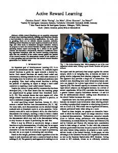
O(MT3 ) + O(MT M 3 ) operations per batch. While this is higher than Algorithm 2, for small M and MT 0) at unobserved θ locations in Θd . For this example, Θd covers the space between −10 ≤ θ1 ≤ 10 and −10 ≤ θ2 ≤ 10 in increments of 0.1 for a total of 40,401 possible sample locations in Θd . It is unlikely Ntotal = 40, 401 in most computationally-constrained scenarios, so the samples must be carefully selected to improve the predictions. 1) Sequential Sampling: First, the sequential sampling procedure from Alg. 1 is demonstrated and compared against existing techniques discussed in Section IV. Additionally, M = 1 versions of the batch procedures in Algs. 2 and 3 are also included for comparison to the sequential algorithm. To illustrate the sampling process, Figures 2 and 3 display one iteration of the for-loop in Algorithm 1. An initial training set of 50 randomly selected samples is used to construct the prediction model shown in Figure 2(a). The (unknown) true model of ρϕ (θ) is shown in Fig. 2(b). The prediction model is used to compute the binary classification entropy shown in Fig. 3. The next training sample is selected according to Eq. 12 from Step 4 of Alg. 1, highlighted as the magenta star. Once the measurement at this θ has been obtained, the prediction model is retrained with this additional information.

Fig. 3: Illustration of binary classification entropy and the selection of sample θ according to Step 4 of Alg 1. The magenta star highlights the selected θ’s location which is then added to training set L. Red/green dots correspond to measurements which indicate failure/satisfaction.

Figure 4 compares the performance of Algorithm 1, averaged over 100 random initializations, against the average performance of existing passive, expected model change (EMC), and variance reduction methods. The prediction error corresponds to misclassifications of ρϕ (θ) > 0 or ρϕ (θ) ≤ 0: whether points that actually satisfy ϕbound were predicted to not satisfy or points that do not satisfy were incorrectly predicted to do so. The sequential entropy-based sampling algorithm outperforms all the other approaches. The approach also outperforms the importance-weighted random sampling procedures from Algs. 2 and 3. Because

only one sample is selected, the k-DPP random matrix theory (RMT) procedure behaves exactly like the baseline importance-weighting algorithm.

Passive EMC Variance: Seq Entropy: Seq Entropy: RMT Entropy: IW

8

Prediction Error (%)

7 6

Passive EMC Variance: RMT Variance: IW Entropy: RMT Entropy: IW

8 7

Prediction Error (%)

Sequential Sampling

9

Batch Size = 5

9

6 5 4 3 2

5

1

4

0 50

100

150

3

200

250

300

350

Samples

2

(a) Mean prediction error (M = 5)

1 0 50

100

150

200

250

300

Samples

2) Batch Sampling: In many applications, it is too computationally-expensive to retrain the GP model after each individual measurement is selected and obtained. In these problems, it is more advantageous to select points in batches of multiple samples and perform simulations at these points all at once. This can also take advantage of parallelization more effectively than sequential algorithms as the simulations can be done in parallel. While it is more efficient, batch sampling must be carefully arranged so as to ensure diversity in the sample set while still selecting relevant points. Section IV-B proposed multiple algorithms based upon binary classification entropy to address those limitations. A comparison of sample selections using Alg. 2 and Alg. 3 for this problem was actually shown earlier in Figure 1. The two approaches were initialized with the same training set and GP model from Fig. 2 and each algorithm forms a relatively large dataset of 30 points. In practice, a such a large number of datapoints is not advised during the initial few iterations because the model changes rapidly with new training batches; however, the figure does effectively illustrate the difference between the two selection processes. The performance of the batch approaches is shown in Figure 5. The two batch algorithms are compared against batch versions of random passive sampling and the EMC algorithm. Two comparable batch versions of the sequential variance reduction method were also developed and their results are plotted in the figure. These batch variance reduction methods are effectively the same as Algorithms 2 and 3 except the probability distribution PH (θ) is instead based upon the current variance Σ(θ) rather than binary classification entropy. The figure illustrates the performance at batch sizes of M = 5 and M = 10 points in each batch. In both plots, the entropy-based sampling methods are shown to outperform the existing techniques. The k-DPP RMT procedure performs slightly better than the baseline importance-weighting technique. This is not unexpected as the comparison in Figure 1 demonstrated that RMT sampling

Passive EMC Variance: RMT Variance: IW Entropy: RMT Entropy: IW

8 7

Prediction Error (%)

Fig. 4: Comparison of entropy-based sampling methods against existing techniques for sequential active sampling. The performance is averaged over 100 different runs with random initializations.

Batch Size = 10

9

350

6 5 4 3 2 1 0 50

100

150

200

250

300

350

Samples

(b) Mean prediction error (M = 10)

Fig. 5: Comparison of batch sampling algorithms at different batch sizes. The performance is averaged over 100 difference runs with random initializations.

would spread the samples more diversely, albeit for an exaggerated case. Regardless, the utility of the entropybased sampling algorithms for simulation-based verification has been established in both sequential and batch sampling settings. 3) Hyperparameter Optimization: As was discussed in Section III-C, the true hyperparameters are not assumed to be known apriori and therefore the hyperparameters must be estimated from the current training set L. Especially during the initial steps of the process, the new measurements obtained the simulation trajectories can drastically differ from the predicted response from the GP model. While the measurements themselves will change the GP prediction model regardless of whether or not the hyperparameters are varied, the new information added by the recent samples can also change the distribution P(σ|yL , θL ) in Eq. 7, requiring the hyperparameters to be re-optimized. The downside of hyperparameter optimization is that it requires multiple O(|L|3 ) operations to obtain a local optimum. In order to illustrate the worth of hyperparameter optimization, Figure 6 compares two versions of Algorithms 2 and 3, one with hyperparameter optimization and one with fixed σ. The results indicate that fixing the hyperparameters when the true/ideal σ are unknown can lead to suboptimal performance, even when active sampling is performed. Note

that since the mean and covariance of GPs are dependent upon the hyperparameters, the entropy will change and the points selected for the next batch will change accordingly. Thus, the training sets will diverge after the first iteration. For both the baseline importance-weighting and RMT procedures with static hyperparameters, the prediction error is actually worse than it was with the initial, smaller training set. After a number of iterations, the prediction error begins to decrease, although this may be due to the fact the size of L begins to become a noticeable larger fraction of the total Θd set. Figure 6 only plots the results for a single batch size of M = 10, but additional runs at various batch sizes and other approaches produced consistent results and behaviors. Batch Size = 10

20 18

Prediction Error (%)

ϕheight = [0,Tf ] (35 − |x[t] − x[0]| ≥ 0),

t ∈[0,Tf ]

14 12 Entropy: IW (Hyp Opt) Entropy: RMT (Hyp Opt) Entropy: IW (Static Hyp) Entropy: RMT (Static Hyp)

10 8 6 4

100

150

200

250

300

350

Samples

Fig. 6: Effect of fixed versus hyperparameter optimization. For the dashed lines, the hyperparameters are held constant from their initial setting while the solid lines depict the procedure where the hyperparameters are re-optimized after each iteration.

B. Heading Autopilot The preceding MRAC example clearly shows that active sampling, in particular active sampling with entropy-based selection metrics, can be used to reduce the prediction error without requiring large numbers of additional samples. The MRAC example is also included because it is 2D and can then be used to easily illustrate the prediction model and closed-loop sampling processes (Figs. 1-3). While the results in the preceding subsection demonstrate between a 75.2 − 77.8% reduction in prediction error from the initial model using entropy-based active sampling, they only demonstrate a 17.5 − 26.4% improvement over existing active sampling procedures. The following example will apply the procedures to a significantly more complex dynamical system and the entropy-based procedures will also demonstrate roughly twice the level of improvement over existing procedures than in the MRAC example. This second example is verification of an aircraft autopilot for controlling lateral-directional flight modes. In particular, the “heading hold” autopilot mode is used to turn the aircraft to and hold a desired reference heading. The simulation model of the autopilot and DeHavilland Beaver airframe is provided by the “Aerospace Blockset” toolbox in Matlab/Simulink [28], [29]. This simulation model includes numerous nonlinearities such as the full nonlinear aircraft dynamics, nonlinear controllers, and actuator models with

(20)

where Tf is the final simulation time and x[t] is the aircraft altitude (in feet) at time t. For this problem, Tf = 50 seconds. The STL robustness metric is similar to the last example with ρϕ (θ) = 0 min ρϕheight [t0 ](θ).

16

2 50

position and rate saturations. The provided “heading hold” autopilot then has several various requirements the closedloop system to satisfy. The requirement chosen for this example is an “altitude hold” requirement of the heading autopilot. In addition to turning the aircraft to the desired heading angle, the autopilot must also ensure the aircraft’s altitude remains within 35 feet of the initial condition when the reference command was given [28], [29]. This requirement can be given in temporal logic form as

(21)

The satisfaction of ϕheight was tested against different initial conditions of the Euler angles, θT =[roll(0), pitch(0), heading(0)]. While satisfaction of other aspects of the heading hold autopilot can be explored, such as heading angle overshoot or steady-state tracking error, the altitude hold requirement dominated the other requirements during an initial trade-space exploration. The space of allowable perturbations ◦ ◦ ◦ ◦ (Θ) spans roll(0) ∈ [−60 , 60 ], pitch(0) ∈ [4 , 19 ], and ◦ ◦ heading(0) ∈ [75 , 145 ]. The desired reference heading was ◦ kept constant at 112 . The discrete sampling set Θd dis◦ ◦ ◦ cretizes Θ into 1 , 0.25 , and 1 increments corresponding to the three Euler angles, resulting in a total of 524,051 possible sampling locations. The performance of the different sampling procedures is shown in Figure 7. For each procedure, these results are averaged over 100 different runs with a randomly selected initial training set of 100 samples. Each procedure starts with the same 100 different training sets as the others. The active learning procedures then select 400 additional training samples out of the remaining |U| = 523, 051 available sample locations. Just as was seen in the previous example, the entropy-based procedures outperform the existing active learning procedures. For both batch sizes (M = 5 and M = 10), the entropy-based procedures produce below 3% prediction error after 500 iterations, about a 40% reduction over the closest variance-reduction method. One important thing to note about this example is that a sequential selection approach like Algs. 1 or 4 is not practical in most computationally-constrained environments when compared to batch methods. Due to the large size of U, re-computation of the variance and entropy after the selection of every sample (O(|L|2 |U|) operations) greatly increases the cost. A comparison of the prediction and training cost for sequential and batch methods is shown in Figure 8. The EMC and importance weighting procedures (for both entropy and variance) all have the same computational cost for training the GP and computing P(ρϕ (θ) > 0), while the RMT methods have a slightly higher cost due to the

Batch Size = 5

11

× 1012 Passive EMC Variance: RMT Variance: IW Entropy: RMT Entropy: IW

9

Prediction Error (%)

8

2

Computational Cost

10

7 6 5 4

1.5

1 Sequential Passive (best case) EMC/IW (M=5) RMT (M=5) EMC/IW (M=10) RMT (M=10)

3 0.5

2 1 0 100

150

200

250

300

350

400

450

500

Samples

Passive EMC Variance: RMT Variance: IW Entropy: RMT Entropy: IW

9

Prediction Error (%)

8 7 6 5 4 3 2 1 150

200

250

300

200

250

300

350

400

450

500

Fig. 8: Comparison of training and prediction costs for the autopilot example. Note that all of these costs do not include the cost of obtaining samples, only the cost of training the GP and computing P(ρϕ (θ) > 0). The cost for “best-case” passive sampling assumes all T samples are taken at once and not sequentially or in batches.

Batch Size = 10

10

0 100

150

Samples

(a) Mean prediction error (M = 5) 11

0 100

350

400

450

500

Samples

(b) Mean prediction error (M = 10)

Fig. 7: Comparison of batch sampling algorithms at different batch sizes applied to the heading autopilot example. The performance is averaged over 100 difference runs with random initializations.

construction of the k-DPP with 1000 samples. All of these approaches are also compared against a “best case” passive procedure, in which all Ntotal samples are obtained before the GP model is constructed. While this passive approach has by far the lowest cost, where 500 passive samples have roughly the same cost as 160 actively-selected samples, the performance is also roughly the same. It is also important to note that the computational cost in Figure 8 does not include the cost of obtaining the samples. As mentioned in Assumption 2, the cost of simulations is assumed to dominate the total cost. VI. C ONCLUSION This work has presented data-driven verification methods for construction of simulation-based certificates of complex nonlinear systems. Given a suitable simulation model of the system, it is relatively straightforward to perform simulations at various uncertainties and use these to predict the system’s ability to satisfy performance requirements. Unlike previous analytical verification techniques, which relied upon the existence of known analytical functions to bound the system’s trajectories, simulation-based methods make no such assumptions and apply to a wider class of systems. The ultimate goal is to construct a statistical certificate

that correctly classifies whether the closed-loop response at particular uncertainties will satisfy the requirements. Methods for converting these qualitative requirements into quantifiable formula were given in Section II. Temporal logic predicates are shown to be a natural approach for expressing the requirements. Signal temporal logic (STL) can be used to produce a single, real-valued, scalar measurement of the satisfaction of the requirements over an entire trajectory. These real-valued measurements not only classify whether the trajectory continuously met all requirements, but also quantify the minimum robustness (or maximum exceedance) at some point in the entire trajectory. A set of the realvalued measurements at different uncertainties is used to construct a Gaussian process (GP) regression model (Section III). This model predicts the STL robustness measurement at unobserved locations along the entire space of feasible uncertainties (Θ). The predicted STL measurements can then be used to estimate whether the corresponding trajectory would in fact satisfy the requirements and also measure the confidence in that estimate. In many applications, the simulations themselves can be computationally expensive to obtain; therefore, it is advantageous to minimize the number of simulations required to obtain accurate predictions. The core of the sample-efficient approach is the active sampling procedures presented in Section IV. All of these procedures utilize binary classification entropy as the metric for selecting future training locations. In addition to a sequential algorithm, two batch sampling algorithms are presented to select multiple training locations at once. These batch methods directly exploit any parallelization in the simulation environment and can be used for additional computational savings. Two examples in Section V demonstrated the improvement in prediction error using the active sampling procedures over other approaches given a limited a number of simulations. Ultimately, data-driven verification procedures are aimed at use within higher-level problems such as robust, nonlinear planning or controller optimization. In those those problems, verification is performed on each candidate control policy

in order to estimate their robustness and the generation of candidate control policies is often an iterative process. Thus, the process would typically cycle through a large number of candidate control policies and it is infeasible to sample the full discretized space of all possible uncertainties for every candidate policy. Sample-constrained data-driven verification aligns with those problems by providing the designer with the best approximation of the robustness while restricted to a budget on the number of allowable simulations during each verification step of the iterative process. While this work has clearly illustrated the potential of data-efficient, simulation-based verification procedures for certification of uncertain nonlinear systems, there remain a few unanswered problems. The focus of this work was on deterministic systems: given the same initial conditions and uncertainties θ, all trajectories and their corresponding STL measurements will be the same. In many applications, stochasticity will be present and can be incorporated into the simulation model. In these problems, trajectories and measurements will no longer be deterministic. Current work in progress has developed similar modeling and sampling procedures for stochastic nonlinear systems, explicitly leveraging the fact multiple measurements can be obtained at each training location. Regardless, the work in this paper presents a clear solution to the problem of computationallyconstrained verification of complex, deterministic nonlinear systems subject to structured uncertainties. R EFERENCES [1] Department of Defense MIL-HDBK-1797, “Flying qualities of piloted aircraft.” [2] Federal Aviation Administration FAR Part 25, “Airworthiness standards: Transport categority airplanes.” [3] E. Lavretsky and K. A. Wise, Robust and Adaptive Control. Springer, 2013. [4] R. S. Sutton and A. G. Barto, Reinforcement Learning: An Introduction. The MIT Press, 1998. [5] J. Moore and R. Tedrake, “Control synthesis and verification for a perching UAV using LQR-trees,” in IEEE Conference on Decision and Control, 2012. [6] S. Prajna, Optimization-Based Methods for Nonlinear and Hybrid Systems Verification. PhD thesis, California Institute of Technology, 2005. [7] J. Kapinski, J. Deshmukh, S. Sankaranarayanan, and N. Arechiga, “Simulation-guided Lyapunov analysis for hybrid dynamical systems,” in Hybrid Systems: Computation and Control, 2014. [8] U. Topcu, Quantitative Local Analysis of Nonlinear Systems. PhD thesis, University of California, Berkeley, 2008. [9] P. Reist, P. V. Preiswerk, and R. Tedrake, “Feedback-motion-planning with simulation-based LQR-trees.” Under review, 2015. [10] J. F. Quindlen, U. Topcu, G. Chowdhary, and J. P. How, “Region-ofConvergence Estimation for Learning-Based Adaptive Controllers,” in American Control Conference, 2016. [11] A. Kozarev, J. F. Quindlen, J. P. How, and U. Topcu, “Case Studies in Data-Driven Verification of Dynamical Systems,” in Hybrid Systems: Computation and Control, 2016. [12] B. Settles, Active Learning. Morgan and Claypool, 2012. [13] O. Maler and D. Nickovic, Monitoring Temporal Properties of Continuous Signals, pp. 152–166. Berlin, Heidelberg: Springer Berlin Heidelberg, 2004. [14] S. Sadraddini and C. Belta, “Robust temporal logic model predictive control,” in Allerton Conference on Communication, Control, and Computing, 2015. [15] D. Sadigh and A. Kapoor, “Safe control under uncertainty with probabilistic signal temporal logic,” in Robotics: Science and Systems Conference, June 2016.

[16] C. Rasmussen and C. Williams, Gaussian Processes for Machine Learning. MIT Press, Cambridge, MA, 2006. [17] J. Kremer, K. S. Pedersen, and C. Igel, “Active learning with support vector machines,” Data Mining and Knowledge Discovery, vol. 4, pp. 313–326, July 2014. [18] Y. Zhang, T. N. Hoang, K. H. Low, and M. Kankanhalli, “Nearoptimal active learning of multi-output gaussian processes,” in AAAI Conference on Artificial Intelligence, 2016. [19] J. F. Quindlen and J. P. How, “Machine Learning for Efficient Sampling-based Algorithms in Robust Multi-Agent Planning under Uncertainty,” in AIAA SciTech Conference, 2017. [20] G. Chen, Z. Sabato, and Z. Kong, “Active learning based requirement mining for cyber-physical systems,” in IEEE Conference on Decision and Control, 2016. [21] A. Gotovos, N. Casati, and G. Hitz, “Active learning for level set estimation,” in International Joint Conference on Artificial Intelligence, pp. 1344–1350, 2013. [22] T. Desautels, A. Krause, and J. W. Burdick, “Parallelizing explorationexploitation tradeoffs in gaussian process bandit optimization,” Journal of Machine Learning Research, vol. 15, pp. 4053–4103, 2014. [23] R. Grande, G. Chowdhary, and J. P. How, “Nonparametric adaptive control using gaussian processes with online hyperparameter estimation,” in IEEE Conference on Decision and Control (CDC), IEEE, 2013. [24] R. Y. Rubinstein and D. P. Kroese, Simulation and the Monte Carlo Method. Wiley, 2008. [25] A. Kulesza and B. Taskar, “Determinantal point processes,” Foundations and Trends in Machine Learning, vol. 5, no. 2-3, pp. 123–286, 2012. [26] A. Kulesza and B. Taskar, “k-dpps: Fixed-size determinantal point processes,” in International Conference on Machine Learning, 2011. [27] G. Chowdhary and E. Johnson, “Concurrent learning for convergence in adaptive control without persistency of excitation,” in IEEE Conference on Decision and Control, IEEE, 2010. [28] C. Elliott, G. Tallant, and P. Stanfill, “An example set of cyber-physical v&v challenges for s5,” in Air Force Research Laboratory Safe and Secure Systems and Software Symposium (S5) Conference, (Dayton, OH), July 2016. [29] C. Elliott, G. Tallant, and P. Stanfill, “On example models and challenges ahead for the evaluation of complex cyber-physical systems with state of the art formal methods v&v,” in Air Force Research Laboratory Safe and Secure Systems and Software Symposium (S5) Conference, (Dayton, OH), June 2015.

VII. A PPENDIX A. Batch Active Sampling using Approximate Entropy Reduction Just as with the sequential algorithm in Alg. 1, the process starts with an initial model and training set L, which is used to compute the entropy (Step 3). The estimated entropy is then initialized to this quantity. Steps 4-8 are the main difference between the sequential procedure and this batch process. Step 5 selects the next sample from the current b estimate of the entropy, H(θ|L∪S, σ). In order to encourage diversity in the points of the batch, this point added to a temporary holding set, S, and removed from U. Set S is then used to update the covariance function Σ(θ) to incorporate the effects of the previously selected points in the batch. The main problem that arises is that the mean function cannot be updated in a similar fashion. The update of µ(θ) would require the measurements ∀θ ∈ S, which have not been obtained at that time. Therefore, the mean is “held” at the training set L, defined as µL (θ), while the covariance is updated with the current S, defined as ΣL∪S (θ). The updated probability of satisfaction is then approximated using the

available information   b+ (θ|L ∪ S, σ) = 1 + 1 erf p µL (θ) P . 2 2 2ΣL∪S (θ)

(22)

The approximate probability of satisfaction can then be used b to compute the estimated entropy H(θ|L ∪ S, σ) in the same manner P+ (θ|L, σ) was used to compute H(θ|L, σ) in Eq. 9 (Step 7). Once a complete batch of M points has been selected, simulations are performed at those locations in S and the corresponding measurements yS are taken (Step 9). Both S and yS are added to the training dataset L and used to retrain the GP model. Once this has been completed, set S is emptied and the process is repeated until T iterations are complete. Algorithm 4 Batch active sampling using approximate entropy reduction 1:

2: 3: 4: 5:

Input: training set L, available sample locations U, trained regression model GP, T batches, M points in each batch, empty set S for i = 1 : T do Compute entropy H(θ|L, σ) ∀θ ∈ U, b set H(θ|L ∪ S, σ) = H(θ|L, σ) for j = 1 : M do b Select θ = argmin H(θ|L ∪ S, σ) θ 0 ∈U

6: 7: 8: 9: 10: 11: 12:

S ← S ∪ θ and U ← U \ θ Update Σ(θ) with θ ∈ S (but not µ(θ)) and b recompute H(θ|L ∪ S, σ) end for Run simulations ∀θ ∈ S, obtain yS L ← L ∪ {S, yS } Reinitialize empty S, retrain GP with new L end for

B. k-Determinantal Point Processes for Sampling Determinantal Point Processes (DPPs) are useful tools for selecting sets of samples where diversity in the samples is important [25]. In these approaches, a set of samples generated according to the underlying probability distribution is used to construct a DPP, which then can be used to produce a second sample set of the same size with a higher level of diversity. In many applications, only a small number of samples are desired; however, the DPP loses its utility when it is constructed from a small number of initial samples. For these problems, k-DPPs [26] were developed to obtain a small set of samples (of size k) from a DPP with a larger initial set of samples. The following algorithm describes kDPP based sampling as it relates to the simulation-based verification procedure. The procedure assumes MT samples of θ have been generated according to PH (θ) formed from the entropy H(θ|L, σ). In order to have a suitable number of samples to construct the DPP, MT ≈ 1000 for the examples in this paper. These samples form a matrix L that measures correlation between samples (Step 4). An isotropic squared

exponential kernel is used to measure similarity and ensure the components of L are L(i, j) ≤ 1 and L is positive definite. The term l is the lone hyperparameter of the RBF kernel. This term was set to l = 5 for the examples. Next, the eigenvalues λj and eigenvectors vj of L are found (Step 7). The eigenvalues are also used to compute the corresponding elementary symmetric polynomials em . These elementary polynomials and the eigenvalues compute the marginal and sampling from marginal in Step 10, adding indices to set J. Once the loop has run out of remaining indices, a sample yi from the set of all indices is chosen and added to Y in Steps 21 and 22. The eigenvector corresponding to yi is then removed from the set V of all remaining eigenvectors. Steps 21-23 are repeated until M samples have been chosen, completing the batch. Note that the values in the output set Y correspond to indices of θ terms in the initial input set of MT θ values sampled from PH (θ). The actual sample locations are taken from that set of MT points. Algorithm 5 k-DPP sampling algorithm; adapted from [26]. 1: 2: 3: 4: 5: 6: 7: 8: 9: 10: 11: 12: 13: 14: 15: 16: 17: 18: 19: 20: 21:

Input: MT randomly generated samples of θ, empty set J, M points in batch for i = 1 : MT do for j = 1 : MT do 2 2 Compute L(i, j) = e−||θi −θj || /l end for end for Eigendecomposition of L → {vj , λj } Initialize m = M for j = MT : −1 : 1 do ej−1 if u ∼ Uniform[0, 1] < λj m−1 then ejm J ← J ∪ {j} m←m−1 if m = 0 then break end if end if end for V ← {vj }j ∈ J Y ←∅ while |V | > 0 do P Select yi with probability P(yi ) = |V1 | v∈V (v T ei )2

Y ← Y ∪ yi V ← V⊥ (orthonormal basis for subspace of V orthogonal to ei ) 24: end while 25: Output: sample set Y of size M 22: 23: