Active learning with evolving streaming data

Active learning with evolving streaming data ˇ Indr˙e Zliobait˙ e1,2 , Albert Bifet2 , Bernhard Pfahringer2 , and Geoff Holmes2 1

Bournemouth University, Poole, UK [email protected] 2 University of Waikato, Hamilton, New Zealand {abifet,geoff,bernhard}@cs.waikato.ac.nz

Abstract. In learning to classify streaming data, obtaining the true labels may require major effort and may incur excessive cost. Active learning focuses on learning an accurate model with as few labels as possible. Streaming data poses additional challenges for active learning, since the data distribution may change over time (concept drift) and classifiers need to adapt. Conventional active learning strategies concentrate on querying the most uncertain instances, which are typically concentrated around the decision boundary. If changes do not occur close to the boundary, they will be missed and classifiers will fail to adapt. In this paper we develop two active learning strategies for streaming data that explicitly handle concept drift. They are based on uncertainty, dynamic allocation of labeling efforts over time and randomization of the search space. We empirically demonstrate that these strategies react well to changes that can occur anywhere in the instance space and unexpectedly.

1

Introduction

Supervised learning models the relationship between the observed variables of an instance and the target variable (label). To build a predictor we need to know the true labels of the training data. Often unlabeled data is abundant but labeling is expensive. Labels can be costly to obtain due to required human input (labor cost). Consider, for example, textual news arriving as a stream. The goal is to predict if a news item will be interesting to a given user at a given time. The interests of the user may change. To obtain training data the historical news needs to be read and labeled as interesting or not interesting. This requires human labor. For instance, Amazon Mechanical Turk3 provides a marketplace for intelligent human labeling. Labeling can also be costly due to a required expensive, intrusive or destructive laboratory test. Consider a production process in a chemical plant where the goal is to predict the quality of production output. The relationship between input and output quality might change over time due to constant manual tuning, complementary ingredients or replacement of physical sensors. In order to know the quality of the output (the true label) a laboratory test needs to be performed which is costly. Under such conditions it may be unreasonable to require true labels for all incoming instances. 3

https://www.mturk.com

2

ˇ I. Zliobait˙ e, A. Bifet, B. Pfahringer, G. Holmes

Active learning studies how to label selectively instead of asking for all true labels. It has been extensively studied in pool-based [14] and online settings [6]. In pool-based settings the decision concerning which instances to label is made from all historical data. In this paper we explore active learning in data stream settings, where this decision needs to be made immediately for every incoming instance, as there is no re-access to it. The main difference between online active learning and active learning in data streams is in expectations around changes. Online active learning typically fixes a threshold (e.g. an uncertainty threshold) and asks for the true label if the threshold is exceeded. In data streams the relationship between the input data and the label may change (concept drift) and these changes can happen anywhere in the instance space. Thus, existing active learning strategies may never query instances from some regions and thus may never know that changes are happening and therefore never adapt. Moreover, in data streams we cannot keep the decision threshold or a region of uncertainty fixed, as eventually the system would stop learning and fail to react to changes. Finally, active learning with data streams must preserve the incoming data distribution to the extent that changes could be detected as they happen. We study active learning strategies specifically for data streams. In brief, the setting is as follows. Data arrives in a stream, and predictions need to be made in real time. Concept drift is expected, thus learning needs to be adaptive. The true label can be requested immediately or never, as the instances are regularly discarded from memory. Our goal is to maximize prediction accuracy over time, while keeping the labeling costs fixed within an allocated budget. After scanning an instance and outputting the prediction for it, we need a strategy to decide, whether or not to query for the true label so that our model could train itself with this new instance. Regular retraining is needed due to changes in data distribution. Active learning strategies in data streams in addition to being able to learn an accurate classifier in stationary situations, need to be able to – balance the labeling budget over time; – notice changes happening anywhere in the instance space; – preserve the distribution of the incoming data for detecting changes; In this paper we develop two such strategies, assuming that the adaptive learning technique is externally given. Experimental evaluation on real data streams demonstrates that the proposed approaches effectively handle concept drift while saving labeling costs as we do not need to label every instance. To the best of our knowledge this study is the first to address active learning for instanceincremental streaming data (we preclude methods that learn from a stream in batches) where historical data cannot be stored in memory. The paper is organized as follows. Section 2 discusses related work. Section 3 presents our active learning strategies for data streams. In Section 4 we analytically investigate the properties of the proposed strategies. Section 5 presents experimental evaluation with real streaming data. Section 6 concludes the study.

Active learning with evolving streaming data

2

3

Related work

Online active learning has been a subject of a number of studies, where the data distribution is assumed to be static [2, 6, 10, 19]. As discussed in the introduction, static online active learning is not designed to handle changes. As we will demonstrate in our analysis and experiments, existing strategies are able to handle drifts if changes happen to be gradual and close to the current decision boundary; however, the reaction to change might be slow. When changes happen far from the decision boundary, such methods fail completely. Those situations require advanced strategies, we develop several such strategies in this study. The problem of label availability in data streams with concept drift has been acknowledged in several recent works [11, 13, 21, 22]. Most convert a stationary active learning or a semi-supervised learning method to an online setting by partitioning a stream into batches and applying stationary strategies within each batch. These works differ from our study in two major aspects. First, their strategies require to inspect a batch of instances at a time, thus they need to assume that limited re-access to data is possible. In contrast, our stream setting requires to make labeling decisions online at the time of scanning each instance. Moreover, the existing active learning or semi-supervised learning strategies only complement concept drift handling strategies, they are not tailored to handle concept drift directly. It is assumed, that the data within a batch is stationary and the goal is to train an accurate classifier, while minimizing labeling costs. Adaptation and drift detection is separate. Thus, these techniques help to learn an accurate current model with fewer labels, but they are not designed to adapt to changes faster or with fewer labels. If changes happen far from the decision boundary, they are likely to be missed. In contrast, we tailor active learning to handle concept drift directly online and search the instance space explicitly. Parts of some of the literature are conceptually related to our approach. We highlight these in the remaining part of this section. The first group uses active learning strategies [16, 17, 24] with batches. Zhu et al. [24] build a classifier on a small portion of data within a batch at random and use uncertainty sampling to label more instances within this batch. A new classifier in each batch is needed to take into account concept drift. Similarly, Masud et al. [17] use uncertainty sampling within a batch to request labels. In addition, they use the unlabeled instances with their predicted labels for training. Lindstrom et al. [16] use uncertainty sampling to label the most representative instances within each new batch. They do not explicitly detect changes, instead they use a sliding window approach, which discards the oldest instances. In summary, these approaches apply static active learning to batches, which is not possible in data streams where historical instances cannot be stored in memory. Note that typically (a real) concept drift refers to changes in the posterior distributions of data p(y|X), where X contains the observed variables and y is the corresponding target variable. In other words, real concept drift means that the unlabeled data distribution does not change, only the class conditional distributions change. In contrast, data evolution refers to changes in the unconditional distribution of data p(X).

4

ˇ I. Zliobait˙ e, A. Bifet, B. Pfahringer, G. Holmes

A few works integrate active learning and change detection [7, 11] in the sense that they first detect change and only if change is detected do they ask for representative true labels. However, only a change in p(X) can be handled this way. We address real concept drift, which means that p(y|X) changes and these changes cannot be detected without labels. Thus, these works are not solving the same problem as our approaches. Additionally, they use pool-based strategies. Another group of works uses semi-supervised learning approaches to label some of the unlabeled data automatically [13, 21, 22]. Klinkenberg [13] separates changes in p(X) from changes in p(y|X) and uses existing semi-supervised techniques to label when p(X) drifts, while a separate non active learning strategy handles changes in p(y|X). Widyantoro and Yen [21] first verify that a concept is stable and only then apply semi-supervised techniques for labeling. Woolam et al. [22] first label some instances within a batch at random and then propagate those labels to other instances using micro clustering. In both works automated labeling concerns only the subsets of the learning problem, which are assumed to be stationary (no real concept drift), which does not correspond to data stream settings we are addressing, thus they are not directly comparable. Two related studies [4, 23] address a slightly different problem, they assume that only a part of the data in a stream is labeled and propose a method to learn from both labeled and unlabeled data. The problem setting is also different from that of this paper, as they do not perform active learning (active labeling). A few works are related to the aspect of variable active learning criterion, which we introduce as a part of our strategies. Attenberg and Provost [2] introduce active inference as an additional aspect of online active learning. They maintain a budget per time period in a stream setting, while instead of uncertainty they estimate the utility of labeling an instance, which also takes into account the expected frequency of seeing a particular instance again. It assumes a possibility of repeated examples. The labeling threshold is fixed, but it depends on more than just uncertainty. This work is limited to the stationary setting. Cesa-Bianchi et al [5] develop an online active learning method for a perceptron based on selective sampling using a variable labeling threshold b/(b + |p|), where b is a parameter and p is the prediction of the perceptron. The threshold itself is based on certainty expectations, while the labels are queried at random. This mechanism could allow adaptation to changes, although they did not explicitly consider concept drift.

3

Strategies

In this Section we present active learning strategies for data streams. We start with two basic techniques and discuss their drawbacks. Then we introduce our strategies in two steps, where each step aims to overcome a challenge posed by the data stream setting. We start with a formal definition of our setting.

Active learning with evolving streaming data

5

Active Learning Framework Input: labeling budget B and strategy parameters 1 2 3 4 5 6 7 8 9

for each Xt - incoming instance, do if Active Learning Strategy(Xt , B, . . .) = true then request the true label yt of instance Xt train classifier L with (Xt , yt ) if Ln exists then train classifier Ln with (Xt , yt ) if change warning is signaled then start a new classifier Ln if change is detected then replace classifier L with Ln

Fig. 1. Strategy framework.

3.1

Setting

Let Xt be an instance, yt its true label, where t indicates the time when an instance arrives. X1 , X2 , . . . , Xt , . . . is then a data stream. The labeling cost is the same for any instance. We impose a budget B to obtain the true labels, which is expressed as a fraction of the number of incoming instances. B = 1 means that all arriving instances are labeled, whereas B = 0.2 means that 20% of the arriving instances are labeled. Figure 1 shows our framework, that combines active learning strategies with adaptive learning. In this work we use the change detection technique of [8]: when the accuracy of the classifier begins to decrease a new classifier is built and trained with new incoming instances. When a change is detected, the old classifier is replaced by the new one. 3.2

Random strategy

The first (baseline) strategy is naive in the sense that it labels the incoming instances at random instead of actively deciding which label would be more relevant. For every incoming instance the true label is requested with a probability B, where B is the budget. See Figure 2 for a formal description. 3.3

Fixed Uncertainty strategy

Uncertainty sampling is perhaps the simplest and the most common active learning strategy [20]. The idea is to label the instances for which the current classifier is the least confident. In an online setting it corresponds to labeling the instances for which the certainty is below some fixed threshold. A simple way to measure uncertainty is to use the posterior probability estimates, output by a classifier. The uncertainty strategy with a fixed threshold is presented in Figure 3.

ˇ I. Zliobait˙ e, A. Bifet, B. Pfahringer, G. Holmes

6

Random(Xt , B) Input: Xt - incoming instance, B -labeling budget. Output: label ∈ {true, false} indicates whether to request the true label yt . 1 2

generate a uniform random variable ξt ∈ [0, 1] return ξt < B

Fig. 2. Random strategy.

FixedUncertainty(Xt , θ, L) Input: Xt - incoming instance , θ - labeling threshold, L - trained classifier. Output: label ∈ {true, false} indicates whether to request the true label yt . 1 2

yˆt = arg maxy PL (y|Xt ), where y ∈ {1, . . . , c} is one of the class labels. return PL (yˆt |Xt ) < θ

Fig. 3. Fixed uncertainty strategy.

3.4

Variable uncertainty strategy

One of the challenges with the uncertainty strategy in a streaming data setting is how to distribute the labeling effort over time. If we use a fixed threshold after some time a classifier would either exhaust its budget or reach the threshold certainty. In both cases it will stop learning and thus fail to adapt to changes. Instead of labeling the instances that are less certain than the threshold we would like to label the least certain instances within a time interval. Thus we introduce a variable threshold, which adjusts itself depending on the incoming data to align with the budget. If a classifier becomes more certain (stable situations), the threshold expands to be able to capture the most uncertain instances. If a change happens and suddenly a lot of labeling requests appear, then the threshold is contracted to query the most uncertain instances first. It may seem counter intuitive that we are asking for more labels at certain situations and fewer labels at changes. In fact, our dynamic threshold assures that we are asking for the same number of labels in all situations. This is how we balance the budget as we do not know when or how often changes will be happening, so we aim to spend the budget uniformly over time. The uncertainty strategy with a variable threshold is described in Figure 4. 3.5

Uncertainty strategy with randomization

The uncertainty strategy always labels the instances that are close to the decision boundary of the classifier. In data streams changes may happen anywhere in the instance space. When concept drift happens in labels the classifier will not

Active learning with evolving streaming data

7

VariableUncertainty(Xt , L, B, s) Input: Xt - incoming instance , L trained classifier, B - budget, s - adjusting step. Output: label ∈ {true, false} indicates whether to request the true label yt . Starting defaults: total labeling cost u = 0, initial labeling threshold θ = 1. 1 2 3 4 5 6 7 8 9 10 11 12 13

if (u/t < B) then budget is not exceeded, yˆt = arg maxy PL (y|Xt ), where y ∈ {1, . . . , c} is one of the class labels. if (PL (yˆt |Xt ) < θ) then uncertainty below the threshold u = u + 1 labeling costs increase, θ = θ(1 − s) the threshold decreases, return true else certainty is good θ = θ(1 + s) make the uncertainty region wider. return false else budget is exceeded return false

Fig. 4. Uncertainty strategy with a dynamic threshold.

notice it without the true labels. In order not to miss concept drift we would like, from time to time, to label the instances about which the classifier is very certain. For that purpose for every instance we randomize the labeling threshold by multiplying by a normally distributed random variable that follows N (1, δ). This way we will label the instances that are close to the decision boundary more often, but occasionally we will also label some distant instances. This strategy trades off labeling some very uncertain instances for labeling very certain instances, in order not to miss changes. Thus, in stationary situations this strategy is expected to perform worse than the uncertainty strategy, but in changing situations it is expected to adapt faster. The uncertainty strategy with randomization is presented in Figure 5. Table 1 summarizes the four strategies with respect to the requirements indicated in the introduction. The random strategy satisfies all three requirements. Randomized uncertainty satisfies budget and coverage, but it produces biased labeled data. The variable uncertainty satisfies only budget and the fixed uncertainty satisfies none.

4

Analysis of how the labeling strategies learn

In this section we explore the main learning aspects of the strategies: the ability to notice changes in dynamic situations and to learn accurate classifiers in stationary situations. In order to demonstrate the behavior of the strategies in controlled settings we employ synthetic data in 2D. The data is distributed uni-

8

ˇ I. Zliobait˙ e, A. Bifet, B. Pfahringer, G. Holmes

VariableRandomizedUncertainty(Xt , L, B, s, δ) Input: Xt - incoming instance , L trained classifier, B - budget, s - adjusting step, δ - variance of the threshold randomization. Output: label ∈ {true, false} indicates whether to request the true label yt . Starting defaults: total labeling cost u = 0, initial labeling threshold θ = 1. 1 2 3 4 5 6 7 8 9 10 11 12 13 14

if (u/t < B) then budget is not exceeded, yˆt = arg maxy PL (y|Xt ), where y ∈ {1, . . . , c} is one of the class labels. θrandomized = θ × η, where η ∈ N (1, δ) is a random multiplier, if (PL (yˆt |Xt ) < θrandomized ) then uncertainty below the threshold u = u + 1 labeling costs increase, θ = θ(1 − s) the threshold decreases, return true else certainty is good θ = θ(1 + s) make the uncertainty region wider return false else budget is exceeded return false

Fig. 5. Uncertainty strategy with randomization. Table 1. Summary of strategies. Controlling Instance space Labeled Data Budget Coverage Distribution Random present full iid Fixed uncertainty no fragment biased Variable uncertainty handled fragment biased Randomized uncertainty handled full biased

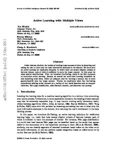
formly at random in a square, the distribution p(X) does not change over time, p(y|X) changes. This data represents a binary classification problem. The initial decision boundary is set at x1 = x2 , as illustrated in Figure 6 (left). Figure 7 shows how the strategies work on the hyperplane problem. The instances that would be labeled by different strategies are visualized. Each strategy labels the same number of instances. The random strategy labels uniformly from the instance space, while the uncertainty strategy concentrates around the decision boundary. The randomized uncertainty infuses randomization into the uncertainty sampling to cover the full instance space. 4.1

Ability to learn changes

Let us look at how concept drift is handled by our strategies. We investigate two situations: a change happening close to the decision boundary, and a re-

Active learning with evolving streaming data

9

change change

original

random

close change remote change

Fig. 6. Data with changes close and far from the decision boundary.

fixed unc.

rand. unc.

Fig. 7. 20% of the true labels queried with different labeling strategies.

mote change. Figure 6 (center and right) presents in black the regions in the instance space that are affected by a change. The center plot illustrates a change that happens close to the decision boundary. The right plot illustrates a remote change. In both examples the number of instances that change is the same. We analyze how well our strategies would notice those changes. Figure 8 (left and center) plots the proportion of the changed (black) instances queried by each strategy. The plots can be interpreted as recall of changes, which is computed as H = qch /Q, where Q is the total number of queried instances and qch is the number of queried instances that have their labels changed. In this evaluation we aim to establish a point in time evaluation thus we do not retrain the classifier after each instance. The fixed uncertainty strategy is omitted, because it does not have a mechanism to control the labeling budget. Besides, the fixed uncertainty strategy handles the changes in the same way as the variable uncertainty strategy, only the budget is handled differently. Comparing the close and the remote change plots we can see, as expected, that the random strategy performs equally well independently of where changes occur. On the other hand, the uncertainty strategy is very sensitive to where changes occur. If changes occur far from the decision boundary, the uncertainty strategy completely misses them and it will never know that the classifier continues making mistakes there. However, the uncertainty strategy captures changes perfectly well if they occur close to the decision boundary, it scores the best of all (100%). The randomized uncertainty reacts to the close changes worse than the uncertainty, but it does not miss the remote changes.

close change

rand. unc.

1

random

0.4 0.2

uncertainty queried

0.8 0.6

recall of uncertainty

remote change 1

uncertainty

recall of changes

recall of changes

1

0.8 0.6 0.4

random rand. unc.

0.2 uncertainty

0 0

0.5 budget

1

0 0

0.5 budget

1

uncertainty

0.8 0.6 0.4

rand. unc. random

0.2 0 0

Fig. 8. Performance of the strategies.

0.5 budget

1

10

4.2

ˇ I. Zliobait˙ e, A. Bifet, B. Pfahringer, G. Holmes

Learning in stationary situations

Active learning strategies in data streams need not only handle changes but also aid the learning to be more accurate. We compare the strategies in terms of queried uncertainty, assuming that the most informative instances in stationary situations lie closest to the decision boundary. Figure 8 (right) plots the queried uncertainty by each strategy against the labeling budget. The plot can be interpreted as recall of uncertainty, P the higher the better. We measure it as u −min u U = 1 − maxq u−min u , where uq = Xqueried pˆ(y|X) is the sum of the posterior probabilities of all the queried instances, min u and max u are the minimum and the maximum possible uq from our dataset. The plot confirms that the variable uncertainty always queries the most uncertain instances, thus it is expected to perform well in stationary situations. The random strategy recalls the least, except for very small budgets, where the variable randomized uncertainty strategy recalls even less. This happens because at small budgets the threshold is very small, therefore nearly all randomization attempts override the threshold and query further away from the decision boundary than random. The variable randomized uncertainty strategy becomes more effective as the budget increases. Notice, that the higher the budget, the more similar the performance, since many of the queried instances overlap.

5

Experimental evaluation

After analyzing our strategies we empirically evaluate their performance along with the baselines. We compare five techniques: random (baseline), fixed uncertainty (baseline), variable uncertainty, variable randomized uncertainty, and Selective Sampling. Our implementation of Selective Sampling is based on [5], and uses a variable labeling threshold b/(b + |p|), where b is a parameter and p is the prediction of the classifier. The threshold is based on certainty expectations, the labels are queried at random. As they did not explicitly consider concept drift, we add change detection to the base classifier to improve its performance. We evaluate the performance on real streaming classification problems. We use as default parameters s = 0.01 and δ = 1. All our experiments are performed using the MOA data stream software suite [3]. MOA is an open source software framework in Java designed for on-line settings as data streams. We use in our experiments an evaluation setting based on prequential evaluation: each time we get an instance, first we test it, and if we decide to pay the cost of its label then we use it to train the classifier. 5.1

Datasets

We use six classification datasets as presented in Table 2. Electricity data [9] is a popular benchmark in evaluating streaming classifiers. The task is to predict a rise or a fall in electricity price (demand) in New South Wales (Australia), given recent consumption and prices in the same and neighboring regions. Cover

Active learning with evolving streaming data

11

Table 2. Summary of the datasets.

Electricity Cover Type Airlines IMDB-E IMDB-D Reuters

instances attributes (nominal + numeric) classes labels 45312 8 (1+7) 2 original 581012 54 (44+10) 7 original 539383 7 (5+2) 2 original 120919 1000 2 assigned 120919 1000 2 assigned 15564 47236 2 assigned

Type data [1] is also often used as a benchmark for evaluating stream classifiers. The task is to predict forest cover type from cartographic variables. As the original coordinates were not available, we ordered the dataset using the elevation feature. Inspired by [12] we constructed an Airlines dataset4 using the raw data from US flight control. The task is to predict whether a given flight will be delayed, given the information of the scheduled departure. IMDB data originates from the MEKA repository5 . The instances are TFIDF representations of movie annotations. Originally the data had multiple labels that represent categories of movies. We construct binary labels in the following way. At a given time we select categories of interest to an imaginary user, the movies of that category get a positive label. After some time the interest changes. We introduce three changes in the data stream (after 25, 50 and 75 thousand instances). We construct two labelings: for IMDB-E (easy) only one category is interesting at a time; for IMDB-D (difficult) five related categories are interesting at a time, for instance: crime, war, documentary, history and biography are interesting at the same time. The Reuters data is from [15]. We formed labels from the original categories of the news articles in the following way. In the first half of the data stream legal/judicial is considered to be relevant (+). In the second half the share listings category was considered to be relevant. The categories were selected to make a large enough positive class (nearly 20% of instances had a positive label). The first three datasets (prediction datasets) have original labels. We do expect concept drift, but it is not known with certainty when and if changes take place. The other three datasets (textual datasets) represent recommendation tasks with streaming data. Every instance is a document in TF-IDF representation. We form the labels of interest from the categories of the documents.

5.2

Results on prediction datasets

We use Naive Bayes as the base classifier for the three prediction datasets. Figure 9 plots the accuracy of a given strategy as a function of the labeling budget. Fixed uncertainty is not included in this figure, since it fails by a large margin. In 4 5

Our dataset is available at http://www.cs.waikato.ac.nz/˜abifet/active http://meka.sourceforge.net/

ˇ I. Zliobait˙ e, A. Bifet, B. Pfahringer, G. Holmes

12

Forest Cover

Electricity

Airlines

0.66 var. unc.

rand. unc.

0.75

sel.

rand. unc.

0.66

0.655 samp. 0.65 var. unc.

0.645 0.64

0

random

random

0.74 0.1

0.2 0.3 0.4 budget used

0.635 0

0.1

0.2 0.3 0.4 budget used

accuracy

0.76

sel. samp.

accuracy

accuracy

0.77

0.665 var. unc. sel. samp.

0.655

rand. unc.

0.65

random

0.645 0.64 0.635 0

0.1

0.2 0.3 0.4 budget used

Fig. 9. Accuracies given a budget on prediction datasets.

the data stream scenario it gives around 50%−60% accuracy, which is equivalent to predicting that all labels are negative. Our strategies (variable and randomized uncertainty) outperform the baseline strategies (random in the plots and the fixed uncertainty not in the plots) and selective sampling as follows. We observe that the variable uncertainty strategy is the most accurate on the Airlines data and on a large part of the Electricity data. In stationary situations or when changes happen close to the decision boundary we expect the variable uncertainty to perform the best. For the Electricity data the randomized uncertainty and the selective sampling perform well at small budgets. That is explainable, as at small budgets variable uncertainty samples only a few instances that are very close to the decision boundary. In such a case randomized uncertainty helps to capture changes better. But as soon as the budget increases, variable uncertainty labels more instances and those include the changes. All the plots exhibit rising accuracy as the budget increases, which is to be expected. If there was no upward tendency, then we would conclude that we have excess data and we should be able to achieve a sufficient accuracy by a simple random subsampling. On the forest cover dataset, randomized uncertainty outperforms the other methods. This learning problem is complex (seven classes), and changes may not happen sufficiently close to the decision boundary, so randomization based methods are best. At small budgets, selective sampling performs well, and when budgets get larger its performance is similar to the random strategy. The variable uncertainty strategy performs well for Airlines, as apparently the data is not changing. The dataset covers only one month, which is a short period for changes to become manifest. Thus randomization of querying strategies does not pay off in this case. Even though more than the minimum number of labels needed, is requested, randomized uncertainty still outperforms the baselines (random and fixed uncertainty). This performance is consistent with our expectations. 5.3

Results on textual datasets

For textual datasets we use the Multinomial Naive Bayes classifier [18]. The classification tasks in these textual datasets are hard and often the results are

Active learning with evolving streaming data IMDB−E

Reuters

IMDB−D rand. unc.

sel. samp.

0.35 var. unc.

0.3 0

0.1

0.2 0.3 0.4 budget used

0.5 random

0.45 sel.

samp.

0.4 var. unc.

0.35 0

0.8 fix. geometric accuracy

rand. unc.

0.4

geometric accuracy

geometric accuracy

random

0.75

unc. rand. unc.

0.2 0.3 0.4 budget used

var. unc.

random

0.7 sel. samp.

0.65 0.1

13

0

0.1

0.2 0.3 0.4 budget used

Fig. 10. Accuracies given a budget on textual drifting datasets.

close to the majority vote, which would mean no recommendation is given by a classifier. Therefore we are interested in balanced accuracy of the classifiers, which is given by the geometric mean GA = (A1 × A2 × . . . Ac )1/c , where Ai is the testing accuracy on class i and c is the number of classes. Note that the geometric accuracy of the majority vote classifier would be zero, as accuracy on the classes other than the majority would be zero. The accuracy of a perfectly correct classifier would be one. If the accuracies of a classifier are balanced across the classes, then the geometric accuracy would be equal to the normal accuracy. Figure 10 presents the geometric accuracies of the three textual datasets. There are several implications following from these results. First, the strategies that use a variable threshold (selective sampling, variable uncertainty, and randomized uncertainty strategy) outperform the fixed threshold strategies (fixed uncertainty), as expected in the data stream setting. Second, the strategies with randomization mostly outperform the strategies without randomization, which suggests that the changes that occur are far from the decision boundaries and there is a justified need for querying tailored to data streams rather than conventional uncertainty sampling. That supports our strategies. Note that as the selective sampling strategy is implemented in our experiments using change detection, it shows good performance on these datasets. However, there is always at least one of the new strategies that outperforms it. On IMDB-E the random strategy performs the best, while on IMDB-D our randomized uncertainty is the best. This different performance can be explained by the nature of the labels. In IMDB-E one category forms the positive label. These categories do not overlap much, as, for instance, science fiction and sports may have little in common. Thus, the decision boundary changes completely and the change occurs far from the decision boundary. Therefore the random strategy is optimal. That is consistent with our simulation findings. In IMDB-D five categories make a positive label at a time. With a larger space for positive labels it is also likely that there is shared vocabulary in the interests before and after the drift. Thus, the drift happens closer to the decision boundary and thus our randomized uncertainty strategy performs better than the fully random one, which is also in line with our reasoning behind the strategies. The randomized uncertainty strategy performs best on the Reuters data as well, while variable

ˇ I. Zliobait˙ e, A. Bifet, B. Pfahringer, G. Holmes geometric accuracy geometric accuracy

14

IMDB−E

change

0.6 0.4

rand. unc.

0.2

random

0

25’000 change

0.6

var. unc. fix. unc.

50’000 75’000 IMDB−D

100’000 rand. unc.

0.4

random var. unc.

0.2

fix. unc.

0

25’000

50’000

75’000

100’000

time

Fig. 11. Progress of accuracies on IMDB drifting datasets.

uncertainty comes second. The changes that are happening may not be that far from each other, the concepts before and after the drift may be related. In the textual datasets we know exactly where the concept drift points are. The progress of the accuracies (prequential) of our strategies and their behavior around the change points Figures 11 and 12. In this active learning experiment we use a fixed 20% budget. From Figure 11 we can clearly see that when more changes happen, the baseline fixed uncertainty fails to react. The variable uncertainty eventually reacts, but slowly. That demonstrates the need for labeling across all the instance space. In Figure 12 we closely inspect the behavior with Reuters data. At the start of learning (left) the strategies that use randomization (random and randomized uncertainty) learn faster. This happens because simple uncertainty strategies learn a classifier from a few points and this classifier becomes very confident about its own predictions and does not require to learn further. At the stable situation (middle) the strategies without randomization perform better than the strategies with randomization, as expected. There are no changes, thus randomization can be seen as a waste of labeling effort. Fixed uncertainty performs well in stable situations, provided its threshold is set appropriately. At change we see that the strategies with randomization react faster than expected. We also see

rand. unc.

random

0.6 var. unc.

0.4 fix. unc.

0.2

geometric accuracy

geometric accuracy

0.8

change

stable

0.9

fix. unc.

1

var. unc.

geometric accuracy

start

0.85 0.8

rand. unc.

0.75

random

0.8

rand. unc.

0.6 var. unc.

0.4 0.2

fix. unc.

random

500

1000 time

1500

2000

0.7

3500

4000 time

4500

5000

0 7000

8000 9000 time

Fig. 12. Progress of accuracies on Reuters dataset.

Active learning with evolving streaming data

15

that the fixed uncertainty strategy fails to adapt. The results at change justifies the need for variable thresholds and randomization of labeling efforts.

5.4

Efficiency

These active strategies reduce the time and space needed for learning, as the classifiers are trained with a smaller number of instances. We can see these active learning strategies as a way to speed up the training of classifiers: only using 30% or 40 % of the instances we may get only a small decrease on accuracy. For example, in our experiments, labeling all instances (B = 1), we see an increase of 5% for the Electricity dataset, 12% for the Cover Type dataset and no increase for the Airlines dataset. On textual data, we obtain an increase of 12% points on the Reuters data set and no change on the IMDB datasets. These results show that these strategies may be a good way to speed up the training process of classifiers. We introduced new strategies for active learning tailored to data streams when concept drift is expected. Different strategies perform best in different situations. Our recommendation is to use the variable uncertainty strategy if mild to moderate concept drifts are expected. If significant drifts are expected then we recommend using randomized uncertainty. In practice we find that drifts can be captured reliably even though the assumption of i.i.d. data is violated.

6

Conclusion

We proposed active learning strategies for streaming data when changes in the data distribution are expected. Our strategies are equipped with mechanisms to control and distribute the labeling budget over time, to balance the labeling for learning more accurate classifiers and to detect changes. Experimental results demonstrate that the new techniques are especially effective when the labeling budget is small. The best performing technique depends on what changes are expected. Variable uncertainty performs well in many real cases where the drift is not that strongly expressed. If more significant drift is expected (as in the textual experiments) then the randomized uncertainty prevails, since it is able to query over all the instance space. This work can be considered as the first step in active learning in the data stream setting. An immediate extension would be to place a grid on the instance space and maintain individual budgets for each region. In such a case it should be possible to dynamically redistribute the labeling budget to the regions where changes are suspected. Acknowledgements. Part of the research leading to these results has received funding from the EC within the Marie Curie Industry and Academia Partnerships and Pathways (IAPP) programme under grant agreement no. 251617.

16

ˇ I. Zliobait˙ e, A. Bifet, B. Pfahringer, G. Holmes

References 1. A. Asuncion and D. Newman. UCI Machine Learning Repository. University of California, Irvine, School of Information and Computer Sciences, 2007. 2. J. Attenberg and F. Provost. Active inference and learning for classifying streams. In n ICML-2010 Workshop on Budgeted Learning, 2010. 3. A. Bifet, G. Holmes, R. Kirkby, and B. Pfahringer. MOA: Massive Online Analysis. Journal of Machine Learning Research, 11(May):1601–1604, 2010. 4. H. Borchani, P. Larranaga, and C. Bielza. Mining concept-drifting data streams containing labeled and unlabeled instances. IEA/AIE (1), 6096:531–540, 2010. 5. N. Cesa-Bianchi, C. Gentile, and L. Zaniboni. Worst-case analysis of selective sampling for linear classification. J. Mach. Learn. Res., 7:1205–1230, 2006. 6. D. Cohn, l. Atlas, and R. Ladner. Improving generalization with active learning. Machine Learning, 15:201–221, May 1994. 7. W. Fan, Y. Huang, H. Wang, and Ph. Yu. Active mining of data streams. In SDM’04, pages 457–461, 2004. 8. J. Gama, P. Medas, G. Castillo, and P. Rodrigues. Learning with drift detection. In SBIA’04, pages 286–295, 2004. 9. M. Harries, C. Sammut, and K. Horn. Extracting hidden context. Machine Learning, 32(2):101–126, 1998. 10. D. Helmbold and S. Panizza. Some label efficient learning results. In COLT ’97, pages 218–230, 1997. 11. Sh. Huang and Y. Dong. An active learning system for mining time-changing data streams. Intelligent Data Analysis, 11:401–419, 2007. 12. E. Ikonomovska, J. Gama, and S. Dzeroski. Learning model trees from evolving data streams. Data Mining and Knowledge Discovery, 23(1):128–168, 2010. 13. R. Klinkenberg. Using labeled and unlabeled data to learn drifting concepts. In IJCAI Workshop on Learning from Temporal and Spatial Data, pages 16–24, 2001. 14. D. Lewis and W. Gale. A sequential algorithm for training text classifiers. In ACM SIGIR, pages 3–12, 1994. 15. D. Lewis, Y. Yang, T. Rose, and F. Li. Rcv1: A new benchmark collection for text categorization research. J. Mach. Learn. Res., 5:361–397, 2004. 16. P. Lindstrom, S. J. Delany, and B. MacNamee. Handling concept drift in a text data stream constrained by high labelling cost. In FLAIRS. AAAI Press, 2010. 17. M. Masud, J. Gao, L. Khan, J. Han, and B. Thuraisingham. Classification and novel class detection in data streams with active mining. In PAKDD’10, pages 311–324, 2010. 18. A. Mccallum and K. Nigam. A comparison of event models for naive bayes text classification. In AAAI Workshop on Learning for Text Categorization, 1998. 19. D. Sculley. Online active learning methods for fast label-efficient spam filtering. In CEAS’07, 2007. 20. B. Settles. Active learning literature survey. Computer Sciences Technical Report 1648, University of Wisconsin–Madison, 2009. 21. D. Widyantoro and J. Yen. Relevant data expansion for learning concept drift from sparsely labeled data. IEEE Tr. on Know. and Data Eng., 17:401–412, 2005. 22. C. Woolam, M. Masud, and L. Khan. Lacking labels in the stream: Classifying evolving stream data with few labels. In ISMIS, pages 552–562, 2009. 23. P. Zhang, X. Zhu, and L. Guo. Mining data streams with labeled and unlabeled training examples. In ICDM’09, pages 627–636, 2009. 24. X. Zhu, P. Zhang, X. Lin, and Y. Shi. Active learning from data streams. In ICDM’07, pages 757–762, 2007.