state or system behaviour at varying levels of rigour and abstraction. It has ..... In this section we present an Object-Z description of a simple ticket machine.
Activity Graphs and Processes Christie Bolton and Jim Davies Oxford University Computing Laboratory Wolfson Building, Parks Road Oxford OX1 3QD {christie,jdavies}@comlab.ox.ac.uk
Abstract. The widespread adoption of graphical notations for software design has created a demand for formally-based methods to support and extend their use. A principal focus for this demand is the Unified Modeling Language (UML), and, within UML, the diagrammatic notations for describing dynamic properties. This paper shows how one such notation, that of Activity Graphs, can be given a process semantics in the language of Communicating Sequential Processes (CSP). Such a semantics can be used to demonstrate the consistency of an object model and to provide a link to other methods and tools. A small example is included.
1
Introduction
The Unified Modeling Language (UML) [RJB97] is a collection of graphical notations, each of which can be used to specify different aspects of structure, state or system behaviour at varying levels of rigour and abstraction. It has been widely adopted for object-oriented software development. UML has an extensively-documented structural semantics but, as [EFLR98] observe, lacks any formal static or behavioural semantics. A significant amount of work has been done on the formal semantics of UML, notably: a type semantics of class models [FBLPS97]; dynamic semantics for state diagrams [LMM99] and state machines [BCR00]; and the combined work of the precise UML group [pUg00]. Closely related to our work is that of [LP99] and [ALBG99]. In addition, some of the notations, being adapted from existing methods, have inherited a formal semantics by association. Activity graphs, diagrams used to describe the flow of behaviour within a system, are an example of this inheritance. They combine features of State Charts [Har87] with the intuition of Petri Nets. The contribution of this paper is two-fold. Firstly we provide a formal semantics for activity graphs, describing them in terms of the process language CSP [Hoa85]. Secondly, based on results presented in [FBLPS97] and a refinementpreserving translation from abstract data types to processes described in [BDW99], and along similar lines to the work of [Fis98] and [BD99], we describe how the final class description of a system can be expressed as an abstract data type and then translated to its corresponding CSP process.
Using refinement we can then compare the process corresponding to a class description against processes corresponding to activity graphs constructed in its development process; we can verify that the final class description is consistent with its specification. An earlier attempt at formalising the semantics of activity graphs, by the current authors, is included in [BD00]. The intent there was quite different: to demonstrate that a uniform process semantics could be used to check the consistency of different parts of a process model. The treatment of activity graphs, in particular, was rather more superficial than that described here. Two notable differences are that the graph transitions in [BD00] could not be labelled with actions and events and that the semantics only applied to graphs with a restricted topology. For instance, the semantics of [BD00] could not cope with cross-synchronisation, as illustrated in Figure 1.
P
Q
R
S
Fig. 1. An activity graph with cross-synchronisation.
In this paper, we take an entirely different approach to the graph notation: states, pseudo-states and transitions are all now modelled in terms of processes. Furthermore, the graph syntax of [BD00] has been discarded and replaced with one much closer to the de facto standard of the Rose interchange format [Rat]. The paper begins with a brief introduction to the mathematical notations used throughout the document. In Section 3, we introduce the graphical notation used in activity graphs and our corresponding syntactic definitions before presenting our behavioural semantics in Section 4. In Section 5, we give an example of a simple class description and an activity graph that might have been constructed during its development process. We show how our behavioural semantics may be used to verify that they are consistent. We conclude the paper with a discussion on the applicability of this work and highlight potential areas for future research.
2
Notation
The mathematical notation used in this paper is a combination of Z [Spi92], CSP [Hoa85] and Object-Z [DRS95,Smi00]. In Section 6 we assume a little knowledge of Petri nets (see, for example, [Pet81]). 2.1
Z and Object-Z
The language of Z is widely used for state-based specification. A characteristic feature is the schema, a pattern of declaration and constraint. The name of a schema can be used anywhere that a declaration, constraint or set could appear. Schemas may be named using the following syntax: Name declaration constraint If S is a schema, then θS denotes the characteristic binding of S in which each declared component is associated with its current value. This semantics supports the definition of a schema calculus, in which specification and analysis can be conducted at the level of schemas, abstracting and encapsulating the components declared within them; we can refer to the collection of identifiers in a particular schema without introducing a named instance of that schema type. Schemas can be used as declarations. For example, the expression λ S • t denotes a function from the schema type underlying S , a set of bindings, to the type of term expression t. The Z notation has a standard syntax for set expressions, predicates and definitions. Basic types, maximal sets within the specification, may be introduced as follows. [Type] Using the axiomatic definition we may introduce a global constant x , drawn from a set S , satisfying predicate p. x :S p Object-Z is an object-oriented extension of Z adding notions of classes, objects, inheritance and polymorphism. A class is represented by a named box containing local types, constant definitions and schemas describing state, initialisation and methods on the class. Class Name[generic parameters] local type and constant definitions state schema initial state schema operations
2.2
Processes
A process, as defined in [Hoa85], is a pattern of communication. We may use processes to represent components in terms of their communicating behaviour, building up descriptions using the standard operators of the CSP language. Processes themselves are defined in terms of events: synchronous, atomic communications between a process and its environment. Compound events may be constructed using ‘ . ’ the dot operator; a family of compound events is called a channel, and may be used to represent the passing of a value between components. Processes may be defined by sets of mutually-recursive equations, that may be indexed to allow parameterised definitions. Parameters may be used to represent aspects of the process state, and may appear in guards: we write B & P to denote the process that behaves as P if B is true, and can perform no events otherwise. The atomic process Skip denotes successful termination, the end of a pattern of communication. If P is a process and a is an event then a → P is a process that is initially ready to engage in a. If this event occurs then the subsequent behaviour is that of P . If P and Q are both processes, then the process P o9 Q first behaves as P and then, if P terminates, behaves as Q. If P and Q are processes, then P � Q represents an internal choice between P and Q: this choice is resolved by the process without reference to its environment. An internal choice over a set of indexed processes {i : I • P (i )} is written � i : I • P (i ). An external choice between two processes, written P 2 Q, may be influenced by the environment; the choice is resolved by the first event to occur. An external choice over a set of indexed processes is written 2 i : I • P (i ); if each begins with a different event, then this is a menu of processes for the environment to choose from. We write � i : I • [A(i ) ] P (i ) to denote an indexed parallel combination of processes in which each process P (i ) can evolve independently but must synchronise upon every event from the set A(i ). The combination may terminate only when every process is ready to do so. In an interleaving parallel combination, no synchronisation is required; in the combination P ||| Q, the two processes evolve independently. We also employ an indexed version of the operator: ||| i : I • P (i ). As with ordinary parallel combination, termination requires the agreement of all parties. Processes may also be partially-interleaved, in the sense that they must synchronise upon certain events but may perform other common events independently. In the combination P |[ A ]| Q, the two processes must synchronise upon every event from the set A, but may perform all others independently. Finally, if P is a process and A is a set of events then P \ A is a process that behaves as P , except that both the requirement to synchronise upon and the ability to observe events from the set A has been removed. 2.3
Behavioural semantics of processes
Several standard semantic models exist for the process language of CSP: see, for example, [Ros98]. For the purposes of this paper we will employ the traces
model; it may be inappropriate to infer precise availability information from an activity graph. In this model, each process is associated with a set of traces, or finite sequences of events. The presence of a trace in the semantic set of a process indicates that it is possible for that process to engage in that sequence of events. Letting Σ denote the set of all event names and CSP denote the syntactic domain of process terms, we may define the semantic function T that takes a CSP process and returns the set of all traces of the given process. T : CSP → � P(seq Σ) The traces model admits a refinement ordering based upon reverse containment. �T
: CSP ↔ CSP
∀ P , Q : CSP • P �T Q ⇔ T (Q) ⊆ T (P ) Refinement may be established through a combination of structural induction [CR99], data-independence [Laz99], and exhaustive, mechanical model-checking as described in [Ros98].
3
Graphical and syntactic descriptions of activity graphs
An activity graph is a special type of state diagram that is used to model the flow of activities within a procedure; essentially it describes a collection of use cases. An activity graph is constructed from a combination of action states, (sub)activity states, start and finish states and pseudostates merge, decision, fork and join. A table showing the graphical representation of each type of state is presented in Figure 2. Syntactically we define these states as follows: Type ::= action
Action�� | activity
ActivityLabel �� | start | finish | merge | decision | fork | join where Action and ActivityLabel are given types. [Action, ActivityLabel ] Note that activity states and action states although graphically indistinguishable, as illustrated in Figure 2, are very different semantically. An action may be thought of as a simple task that cannot be broken down any further, whereas an activity is a task that can be broken down, and may itself be expressed as an activity graph. An ActivityLabel within an activity state points to another activity graph within the specification; an example of an activity state is “Build House” within the “Create House” activity graph illustrated in Figure 3. The states within an activity graph are linked together by transition lines. These lines may have associated guards and actions as illustrated in Figure 4.
action
activity
start
�? � �? � �
� �
~
�
merge
decision
? �HH -� H � H�
? ��HH H � H�
?
?
? w n
?
?
?
finish
fork
join
? ?
? ?
? ?
Fig. 2. States of an activity graph.
Given the types Line and Guard , [Line, Guard ] the schema definition of a transition is as follows: Transition guard : Guard action : Action line : Line If the graphical representation shows no guard or no action then the schema description of the transition records the default values true and null respectively. true : Guard null : Action Each state within an activity graph records the type of its contents, the set of incoming lines it requires and the set of outgoing transitions it enables. State lines : P Line transitions : P Transition type : Type The type State allows all possible states, including those which are not permissible within a UML specification. The schema WellFormed describes the subset
Create House
Build House
Lay Foundations Draw up Plans Build Walls Build House
Install Electricity
Decorate
Put on Roof
Fig. 3. A graph nested within a graph.
[ guard ]
action
Fig. 4. A simple transition, a guarded transition, and a transition enabled by an action.
of possible states that are permissible according to the constraints within the official documentation [OMG99]. WellFormedState State type = start ⇔ lines = ∅ type = finish ⇔ transitions = ∅ type ∈ {start, merge, join} ⇒ #transitions = 1 type ∈ {finish, decision, fork } ⇒ #lines = 1 ( ∃ tr : transitions • tr .line ∈ lines ) ⇒ type �∈ {start, finish, merge, decision, fork , join}
An activity graph is built up from a finite set of well-formed states. The environment of a specification is a function mapping the name of each graph to the associated graph. These are described formally below. Graph ::= states
F WellFormedState �� Env == ActivityLabel → � Graph
4
Behavioural and semantic descriptions
In this section we define our semantic function which takes the name of an activity graph within a specification and returns the CSP process that models the behaviour of that graph. Essentially, this function returns the parallel combination of the processes corresponding to the states within the named graph each synchronising on its own alphabet; the synchronisation of the line events ensures that the actions occur in the correct order. We introduce the types Process and Event [Process, Event] and define the functions εline and εaction which, respectively, map line names and actions to events. We insist that events corresponding to each line and to each action are distinct. Having defined an Action to be a simple task that cannot be broken down any further we may justifiably model it as a single event. εline : Line � � Event εaction : Action � � Event ran εline ∩ ran εaction = ∅ 4.1
Alphabets
In order to define the alphabet for each state—the events on which it must synchronise—we must consider the events associated with each line, type and transition. We introduce functions αline , αtran , αtype and αstate which respectively take a line, a transition, the type of a state, and a state and return the associated set of events. The set of events associated with a line is simply the relational image of the line under εline . The set of events associated with a transition is the set containing the events corresponding to its line and its action. αline : Line → � P Event αtran : Transition → � P Event αline = ( λ line : Line • {εline line} ) αtran = ( λ Transition • { εline line, εaction action } ) The set of events associated with the type action state with given action actn is the set containing the singleton event corresponding to actn, whereas the set of events associated with the type activity state with given ActivityLabel actL is the alphabet of the graph corresponding to actL; this is simply the union of the alphabets of all the states in the identified graph. The set of events associated with all other types of state is simply the empty set.
αtype : Type → � Env → � P Event ∀ env : Env ; type : Type; actn : Action; actL : ActivityLabel • type ∈ {start, finish, merge, decision, fork , join} ⇒ αtype type env = ∅ ∧ αtype (action actn) env = {εaction actn} ∧ � αtype (activity actL) env = ( { state : State | state ∈ states ∼ (env actL) • αstate state env } ) The alphabet of a given state is the union of the alphabets of all of its incoming lines, the alphabet of its type and the alphabets of all of its outgoing transitions. αstate : State → � Env → � P Event αstate = ( λ State • � ( λ env : Env • ( (αline (| lines |)) ∪ � (αtran (| transitions |)) ∪ αtype type env ) ) ) 4.2
Processes
We observed at the beginning of Section 4 that the process corresponding to the behaviour of a named activity graph within its specification environment was simply the parallel combination of the processes corresponding to its constituent states, each synchronising on its own alphabet. All line events are then hidden. We formally define the function as follows. semantics : ActivityLabel → � Env → � Process ∀ env : Env ; actL : ActivityLabel • semantics actL env = (� state�: states ∼ (env actL) • [ αstate state env ] ρstate state env ) \ ( {st : states ∼ (env actL) • εline (| st.lines |)} ) The function ρstate returns the process corresponding to the behaviour of the given state. ρstate is essentially the sequential composition of the processes corresponding to the lines, type and transitions of the given state. In order define it formally we must consider these constituent processes and the effect of loops on the system. The process that corresponds to the behaviour of the type action state with given action actn, is simply the event associated with actn followed by Skip,
whilst the process that corresponds to the behaviour of the type activity state with given ActionLabel actL, is the process corresponding to the graph associated with actL. The process that corresponds to the behaviour of all other types of states is simply Skip. ρtype : State → � Env → � Process ∀ state : State; env : Env ; actn : Action; actL : ActivityLabel • state.type = action actn ⇒ ρtype state env = (εaction actn) → Skip ∧ state.type = activity actL ⇒ ρtype state env = semantics (actL) env ∧ state.type ∈ {start, finish, merge, decision, fork , join} ⇒ ρtype state env = Skip We observe that the difference between a merge state and a join state is that a merge state can be reached provided any one of its incoming lines is enabled whereas a join state can be reached only when all of its incoming lines have been enabled. In order to reflect these differences we define the following processes. RequireAny(ls) = RequireAll (ls) =
2 e : εline (| ls |) • e → Skip ||| e : εline (| ls |) • e → Skip
Similarly, in order to reflect the difference between a fork state where all outgoing transitions are enabled and other states where only one transition may be chosen, we define the following processes. Fork (ts) =
||| Transition | θTransition ∈ ts •
guard & ( if (action = null ) then (εline line) → Skip else (εaction action) → (εline line) → Skip ) )
Choice(ts) =
2 Transition | θTransition ∈ ts •
guard & ( if (action = null ) then (εline line) → Skip else (εaction action) → (εline line) → Skip ) )
Observe that if there is no action event on the transition line, that is action = null , then the corresponding process has no action event. Given these definitions we define the function ρtrans that takes a state and returns the process that corresponds to the behaviour of its outgoing transitions:
ρtrans : State → � Process ρtrans = ( λ State • if (component = finish) then Skip else if (component = fork ) then Fork (transitions) else Choice(transitions) ) Note that we define the process corresponding to the transitions of a finish state to be Skip. This avoids having to choose one from an empty set of transitions that would give rise to deadlock. Before we define the function ρlines , consider the graph illustrated in Figure 5. Since line2 is a self-transition, that is, it loops back directly to the same state,
line1
line2 actn
Fig. 5. An activity looping back to itself.
the event εline line2 will not be in the alphabet of the process corresponding to any other state. This event will therefore not be constrained by synchronisation and can occur at any time. Thus, we must treat incoming lines which are part of a self-transition separately when considering the process corresponding to the incoming lines. We define the function loops to take a state and return the set of all self-transitions, and the function αloops to return the set of all lines contained in a self-transition. αloops : State → � P Event loops : State → � P Transition loops = ( λ state : State • {tr : state.transitions | tr .line ∈ state.lines } ) αloops = ( λ state : State • {tr : loops state • εline (tr .line)} ) Given these definitions, and recalling that only action states and activity can have direct loops back to themselves in a well-formed graph, we define the function ρlines which takes a state and returns the process describing the behaviour of all the incoming lines as follows. ρlines : State → � Process ρlines = ( λ state : State • if (type = join) then RequireAll (lines) else RequireAny(lines \ (αloops state)) )
Finally, we define the function ρstate which takes a state within a given specification environment and returns the process which models the behaviour of the entire state; the incoming lines, the type of state and the outgoing transitions. ρstate : State → � Env → � Process ρstate = ( λ state : State • ( λ env : Env • if (type = start) then ρtrans state else if (αloops state = ∅) then let X = ρlines state o9 ( ρtype state env ρtrans state o9 X ||| X) within X else let Y = ρlines state o9 (Z ||| Y ) Z = ρtype state env o9 ( Choice (loops state) o9 Z 2 Choice (transitions \ (loops state)) o9 Y ) within Y )) Observe that the process corresponding to a start state is the only non-recursive process; a start activity can occur only once. For all other states, through interleaving the process with itself after the events corresponding to the incoming lines have occurred, we enable the incoming lines events to occur many times before the events corresponding to the state type and the state transitions occur1 , thereby mirroring the intended behaviour of the graph and hence the system.
5
Example
In this section we present an Object-Z description of a simple ticket machine. We assume that this model was derived as the result of a UML specification and present an activity graph that might have been constructed in the development process. We show how both the Object-Z description and the activity graph can be translated to their process equivalents in CSP. We are then able to do a refinement check to determine whether or not the final model is consistent with the activity graph. 1
This corresponds closely to Petri nets in which each place can contain multiple tokens.
5.1
Activity graph describing a ticket machine
We assume that the activity graph illustrated in Figure 6 was constructed during the development process of a ticket machine (although we have added line names to our graph). We observe that a coin can be inserted at any time, and that for line1
Insert Coin line2
line4
line3 line5 green
line6
line9 red
Issue Ticket line7
line8 line10
Return Coin
Fig. 6. An activity graph describing a simple ticket machine.
each coin that has been inserted either the red button or the green button may be pressed. If the red button is pressed then a coin will be returned. If the green button is pressed then the machine will non-deterministically choose either to issue a ticket or to return a coin. We define the following set I which indexes the processes corresponding to the states within the graph. I = {start, insert, fork , choice1, choice2, return, issue, stopR, stopG} In addition, we identify the following sets of events corresponding to the actions and lines described in the graph. Actions = {insertCoin, pressRed , pressGreen, issueTicket, returnCoin} Lines = {l : 1 . . 10 • line.l } Our syntax corresponds closely to the Rational Rose interchange format [Rat] and we may therefore readily obtain our syntactical interpretation of the graph. Applying our semantic function to this syntactic description we obtain the process corresponding to the activity graph. GraphProcess = ( � i : I • [ A(i ) ] P (i ) ) \ Lines where for each i in I , the process P (i ) is as defined below: P (start) = line.1 → Skip
P (insert) = (line.1 → Skip 2 line.4 → Skip) o9 ( insertCoin → line.2 → P (insert) ||| P (insert) ) P (fork ) = line.2 → ( ( line.3 → Skip ||| line.4 → Skip ) o9 P (fork ) ||| P (fork ) ) P (choice1) = line.3 → ( green → line.5 → P (choice1) 2 red → line.9 → P (choice1) ||| P (choice1) ) P (choice2) = line.5 → ( line.6 → P (choice2) 2 line.8 → P (choice2) ||| P (choice2) ) P (issue) = line.6 → ( issueTicket → line.7 → P (issue) ||| P (issue) ) P (stopG) = line.7 → (Skip ||| P (stopG)) P (return) = (line.8 → Skip 2 line.9 → Skip) o9 ( returnCoin → line.10 → P (return) ||| P (return) ) P (stopR) = line.7 → (Skip ||| P (stopR)) and for each i in I , the set of events A(i ) is as defined below: A(start) = {line.1} A(insert) = {line.1, line.2, line.4, insertCoin} A(fork ) = {line.2, line.3, line.4} A(choice1) = {line.3, line.5, line.9, red , green} A(choice2) = {line.5, line.6, line.8} A(issue) = {line.6, line.7, issueTicket} A(stopG) = {line.7} A(return) = {line.8, line.9, line.10, returnCoin} A(stopR) = {line.10}. 5.2
Object-Z description of a ticket machine
In this section we give an Object-Z description of a ticket machine which might have been constructed based on a UML specification containing the activity graph illustrated in Figure 6.
Four state variables have been introduced during the development process: coins is the number of coins that have been inserted for which the user has not yet selected the red button or the green button; tickets is the number of tickets left in the machine; toReturn is the number of coins to be returned; and toIssue is the number of tickets to be issued. Note that the non-determinism in the activity graph—the machine could either return a coin or issue a ticket if the green button was pressed—has been resolved. In the Object-Z description, if the green button is pressed then the machine will issue a ticket if there is one left; otherwise it will return a coin. TicketVendingMachine coins, tickets : N toReturn, toIssue : N
Init coins = 0 toReturn = toIssue = 0
InsertCoin ∆(coins)
PressRed ∆(coins, toReturn)
coins � = coins + 1
coins � = coins − 1 toReturn � = toReturn + 1
PressGreen ∆(coins, toIssue, toReturn) coins � = coins − 1 ( toIssue � = toIssue + 1 ∧ toReturn � = toReturn ∨ toIssue � = toIssue ∧ toReturn � = toReturn + 1 )
IssueTicket ∆(toIssue)
ReturnCoin ∆(toReturn)
toIssue � = toIssue − 1
toReturn � = toReturn − 1
Applying the methods described in [BD00] for translating a Z or Object-Z description, via an abstract data type to its corresponding process, and invoking the theorem presented in [BDW99] that this translation preserves refinement: Theorem One abstract data type is refined by another precisely when the process corresponding to the first is refined by the process corresponding to the second.
we see that the process corresponding to our Object-Z description is described by ClassDescProcess below. ClassDescProcess = let P (c, t, iss, ret) = insertCoin → P (c + 1, t, iss, ret) 2 c > 0 & red → P (c − 1, t, iss, ret + 1) 2 c > 0 & green → ( if t > 0 then P (c − 1, t, iss + 1, ret) else P (c − 1, t, iss, ret + 1) 2 iss > 0 & issueTicket → P (c, t − 1, iss − 1, ret) 2 ret > 0 & returnCoin → P (c, t, iss, ret − 1) within � t : {0 . . T } • P (0, t, 0, 0) The integer T is the machine’s ticket capacity. On initialisation it may be filled with any number of tickets not exceeding that capacity. Initially no coins have been inserted, no coins need returning and there are no tickets waiting to be issued. 5.3
Verifying consistency
We prove that our final model of a ticket machine is consistent with the activity graph constructed in its development process using refinement. In attempting to analyse a UML specification, we must take account of the context in which each diagram is presented. In general, activity graphs are intended only to illustrate a particular use case and so it would be inappropriate to infer availability information; hence we use the traces model to compare GraphProcess with ClassDescProcess. ClassDescProcess �T GraphProcess This refinement check tells us that every sequence of methods allowed by the activity graph is a possible behaviour of the class description. For specifications in which the activity graph is intended to convey availability information, we would use the stable failures refinement [Ros98] rather than the traces model employed here.
6
Adequacy and application
Whilst the processes corresponding to our activity graphs defined in Section 4 and illustrated in the ticket machine example in Section 5 are entirely correct
they cannot in practise be used we come to analysing the system using a model checker. The interleaving of the process corresponding to each state with itself causes the system to diverge. This interleaving is, however, necessary if, for instance, we wish to allow the user of the ticket machine to be able to insert two coins before they press either the red or the green button. To eliminate divergence we must, in Petri net terms, put an upper limit on the number of tokens allowed in any place; that is, for each action state and activity state we must only allow a finite number of events corresponding to an incoming line to occur before an event corresponding to an outgoing transition occurs. We extend the definition of State to incorporate the variables isDynamic and dynamicMultiplity as defined in the official documentation [OMG99]. The Boolean isDynamic is True for action states and activity states in which the state’s actions may be executed concurrently. If this Boolean is True then the integer dynamicMultiplicity limits the number of parallel executions of the actions of the state. If the Boolean isDynamic is False, then dynamicMultiplicity is ignored. PracticalState WellFormedState isDynamic : Bool dynamicMultiplicity : N type ∈ {start, finish, merge, decision, fork , join} ⇒ isDynamic = False We define the functions inComing and outGoing which take a PracticalState and return respectively the set of events corresponding to the incoming non-looped lines and the set of events corresponding to the lines within the non-looped outgoing transitions. Given these definitions, we define the function constraint which returns the process which limits the number of parallel executions of each state. inComing : PracticalState → � P Event outGoing : PracticalState → � P Event constraint : PracticalState → � Process ∀ state : PracticalState • inComing state = εline (| state.lines |) \ αloops state outGoing state = {tr : state.transitions • εline (tr .line)} \ αloops state constraint state = let Con(n) = (n < state.dynamicMultiplicity) & 2 in : inComing state • in → Con(n + 1) 2 2 out : outGoing state • out → Con(n − 1) within Con(0)
Using these definitions, the process that, for practical purposes, we should use to model the behaviour of each state is given below. ρpractical
state
: PracticalState → � Env → � Process
ρpractical state = ( λ state : State • ( λ env : Env • if (isDynamic = False) then ρstate state env else ρ state env |[ (inComing state) ∪ (outGoing state) ]| constraint state Hence it follows that, for practical purposes, our semantic function should be semanticsP : ActivityLabel → � EnvP → � Process ∀ env : EnvP ; actL : ActivityLabel • semantics actL env = (� stateP : statesP ∼ (env actL) • [ αstate stateP env ] ρpractical state stateP env ) � \ ( {stp : statesP ∼ (env actL) • εline (| stp.lines |)} ) where a EnvP maps activity labels onto “practical” graphs and where practical graphs are a collection of PracticalStates. EnvP == ActivityLabel → � GraphP GraphP ::= statesP
F PracticalState ��
7
Discussion
The Unified Modeling Language has many strengths. For instance, its graphical nature makes it easily readable by domain experts without a formal mathematical training; as such it provides a common ground for discussing the behaviour of the system to be developed. In addition, the combination of notations allows the user to reason at different levels of rigour and abstraction and from both behavioural and state-based perspectives. However, as [EFLR98] observe, before UML can earn its place as a de facto standard for modelling object-oriented systems it must have a precisely defined semantics, and not just the precisely defined syntax that it has at present. In this paper we have presented a formal behavioural semantics for activity graphs. We have illustrated, using a simple example, how this semantic model may be used to verify that the behaviour of the final class model description of a system is consistent with the behaviour of activity graphs constructed during its development process. In addition, we have considered the practicalities of integrating such a semantics into a modelling tool; our syntax corresponds closely to the Rose interchange format [Rat], and we have built constraints into our practical model which will prevent the system from diverging.
A considerable amount of work remains to be done both in this particular area and in the wider scope of UML. In the semantics presented in this paper we have built guards into our model, but have not gone into detail as to how they should be used. At present we have adopted the most simplistic approach in which each guard is a constant value: null or True or False. An interesting area of research would be to consider how to model guards which are dependent on state variables and the effect that this would have on activity graphs with loops and multiple threads. In addition, using the behavioural semantics presented here to verify consistency relies on the assumption that we can translate the final class model to an abstract data type and hence to its process equivalent. However the example we presented was a simple one with a single class. In theory a single class example is sufficient; [FBLPS97] shows that formal descriptions of models with multiple classes and associations can be constructed by promoting the data types that model the individual classes. The process of reasoning about these descriptions can then be simplified: [WD96] explains in some detail how refinement distributes through promotion. However, we need to consider larger, more complex examples to check that this method is scalable and practicable. Finally, it would be interesting to see if we could link the work presented here with that of [Fis00]. Such a link would facilitate the automatic verification of consistency between activity graphs and the final java code. Whilst these issues still need to be addressed, it is our hope that the work presented in this paper, combined with the work done by many others in this area, will lead to the automatic verification by modelling tools of the preservation within the final class description of both the static and behavioural properties captured in UML diagrams.
Acknowledgements We would like to thank Jim Woodcock, Perdita Stevens and Geraint Jones for their helpful and insightful comments.
References [ALBG99] D. Amyot, L. Logrippo, R.J.A. Buhr, and T. Gray. Use case maps for the capture and validation of distributed systems requirements. In Proceedings of RE ’99, 1999. [BCR00] E. B¨ orger, A. Cavarra, and E. Riccobene. Modeling the dynamics of UML state machines. In Y. Gurevich, P. Kutter, M. Odersky, and L. Thiele, editors, Proceedings of ASM’00, LNCS. Springer-Verlag, 2000. [BD99] H. Bowman and J. Derrick. A junction between state-based and behavioural specification. In P. Ciancarini, A. Fantechi, and R. Gorrieri, editors, Proceedings of FMOODS ’99. Kluwer, 1999. [BD00] C. Bolton and J. Davies. Using relational and behavioural semantics in the verification of object models. In C. Talcott and S. Smith, editors, Proceedings of FMOODS ’00. Kluwer Academic Publishers, 2000. To appear.
[BDW99]
C. Bolton, J. Davies, and J. Woodcock. On the refinement and simulation of data types and processes. In K. Araki, A. Galloway, and K. Taguchi, editors, Proceedings of IFM’99. Springer, 1999. [CR99] S. J. Creese and A. W. Roscoe. Verifying an independent family of inductions simultaneously using data independence and fdr. In Proceedings of FORTE/PSTV ’99. Kluwer Academic Press, 1999. [DRS95] R. Duke, G. Rose, and G. Smith. Object-Z: a specification language advocated for the description of standards. Computer Standards and Interfaces, 17:511 – 533, 1995. [EFLR98] A.S. Evans, R.B. France, K.C. Lano, and B. Rumpe. Developing the UML as a formal modelling notation. In J. Bezivin and P.-A. Muller, editors, UML’98 - Beyond the notation, volume 1618 of LNCS. Springer, 1998. [FBLPS97] R. B. France, J.-M. Bruel, M. M. Larrondo-Petrie, and M. Shroff. Exploring the semantics of UML type structures with Z. In H. Bowman and J. Derrick, editors, Proceedings of FMOODS ’97, volume 2. Chapman and Hall, 1997. [Fis98] C. Fischer. How to combine Z with a process algebra. In J. Bowen, A. Fett, and M. Hinchey, editors, Proceedings of ZUM ’98, volume 1493 of LNCS. Springer-Verlag, 1998. [Fis00] C. Fischer. Combination and implementation of processes and data: from csp-oz to java. PhD thesis, University of Oldenburg, 2000. [Har87] D. Harel. Statecharts: A visual formalism for complex systems. Science of Computer Programming, 8, 1987. [Hoa85] C. A. R. Hoare. Communicating Sequential Processes. Prentice Hall, 1985. [Laz99] R. Lazic. A semantic study of data independence with applications to model checking. PhD thesis, University of Oxford, 1999. [LMM99] D. Latella, I. Majzik, and M. Massink. Towards a formal operational semantics of UML statechart diagrams. In A. Fantechi P. Ciancarini and R. Gorrieri, editors, Proceedings of FMOODS ’99. Kluwer, 1999. [LP99] J. Lilius and I. Porres Paltor. Formalising UML state machines for model checking. In R. France and B. Rumpe, editors, UML’99 - The Unified Modeling Language, volume 1723 of LNCS. Springer, 1999. [OMG99] Object Management Group. Unified Modeling Language Specification, version 1.3. Rational Software Corporation, Santa Clara, CA 95051, USA, June 1999. [Pet81] J. L. Peterson. Petri Net Theory and the Modeling of Systems. Prentice-Hall International, 1981. [pUg00] precise UML group. http://www.cs.york.ac.uk/puml/, 2000. [Rat] Rational Software Corporation, Santa Clara, CA 95051, USA. Rational Rose. http://www.rational.com/products/rose. [RJB97] J. Rumbaugh, I. Jacobson, and G. Booch. The Unified Modeling Language reference manual. Addison-Wesley, 1997. [Ros98] A. W. Roscoe. The Theory and Practice of Concurrency. Prentice Hall Series in Computer Science, 1998. [Smi00] G. Smith. The Object-Z specification language. Kluwer Academic Publishers, 2000. [Spi92] J. M. Spivey. The Z notation: a reference manual. Prentice-Hall International, 1992. [WD96] J. C. P. Woodcock and J. Davies. Using Z: Specification, Proof and Refinement. Prentice Hall International Series in Computer Science, 1996.