The optical ow estimation is not an exception to this rule 5, 9, 10, 19, 21, 25]. ..... 78s. M6;4;2. 4:75o. 6:89o. 92s. Adaptive grids model cpu. M6. 5:09o. 7:20o. 28s.
INSTITUT NATIONAL DE RECHERCHE EN INFORMATIQUE ET EN AUTOMATIQUE
Adaptative Multigrid and Variable Parameterization for Optical-flow Estimation
Etienne M´emin and Patrick P´erez
N ˚ 3102 Janvier 1997
` THEME 3
ISSN 0249-6399
apport de recherche
Adaptative Multigrid and Variable Parameterization for Optical- ow Estimation Etienne M�emin and Patrick P�erez Th�eme 3 | Interaction homme-machine, images, donn�ees, connaissances Projet Temis Rapport de recherche n�3102 | Janvier 1997 | 19 pages
Abstract: We investigate the use of adaptative multigrid minimization algorithms for the estimation
of the apparent motion eld. The proposed approach provides a coherent and e�cient framework for estimating piecewise smooth ow elds for di�erent parameterizations relative to adaptative partitions of the image. The performances of the resulting algorithms are demonstrated in the di�cult context of a non convex global energy formulation.
Key-words: optic ow, robust statistics, global minimization, adaptative grids, multigrid algorithms, variable parameterization
(R�esum�e : tsvp)
Algorithme multigrille adaptatif et param�etrisation variable pour l'estimation du ot optique R�esum�e : Nous pr�esentons une famille d'algorithmes de minimisation, multigrilles et adaptatifs, de-
di�es �a l'estimation du champs des vitesses apparentes dans une s�equence d'images. Ce sch�ema de minimisation est d�ecrit de mani�ere g�en�erale pour di��erentes param�etrisations du champ des vitesses. La formulation uni �ee ainsi obtenue conduit de fa�con naturelle et coh�erente �a estimer sur une partition adapt�ee de l'image un champ comme fonction continue par morceaux avec divers degr�es concomittants de param�etrage.
Mots-cl�e : ot optique, statistique robuste, minimisation globale, grilles adaptatives, algorithmes multigrilles, param�etrisation variable
1 Introduction Energy-based models constitute a powerful way to cope with low-level image processing problems. Those methods are issued either from continuous formalisms such as PDEs or either from discrete modelization such as Markov random elds. The underlying problems are easily tractable if the energy is convex. One has then to deal with functions having an unique minimum that may be estimated with deterministic descent minimization algorithms. However, when it comes to design accurate and robust methods, able to handle and to locate as precisely as possible discontinuities, energies tend to be non linear with numerous local minima. The optical ow estimation is not an exception to this rule [5, 9, 10, 19, 21, 25]. Even within an incremental multiresolution formulation of the problem (which is almost inescapable in case of long range motions to be estimated), one has to deal with a sequence of global optimization problems which remain tricky. To cope e�ciently with such global energy minimization, we propose here a family of deterministic optimization algorithms. These multigrid algorithms are extensions of the method proposed in [21]. They allow to properly combine a multigrid minimization strategy with the mutiresolution framework commonly used in motion analysis. The key idea consists in the minimization of the energy function through an appropriate hierarchy of subspaces of the whole con guration space. Each subspace is de ned as a set of con gurations constrained to be piecewise parametric relative to a certain partition of the image. These multigrid minimization algorithms turn out to provide an accelerated convergence toward improved estimates. Furthermore, associated to a dense robust optic ow estimation model, the multigrid framework provides e�cient motion estimators allowing to combine di�erent parameterizations of the velocity eld through an adaptative partition of the image grid. A compromise solutions between local dense methods [5, 16, 21] involving smothness constraints and global parametric approaches assuming low order polynomial representation of the velocity eld [1, 2, 4, 7] is thus introduced. The remainder of the paper is organized as follows. In section 2, we present the robust motion estimation framework of interest. The estimation is presented as the incremental minimization of a global energy function. The objective function considered here, involves robust estimators to deal both with spatial discontinuities of the velocity eld and with large deviations from the data model. In section 3, we present the proposed multigrid framework. Our approach is validated qualitatively and quantitatively on real world and synthetic sequences. These experimental results are reported in section 4.
2 Robust incremental estimation Standard optical- ow estimators are based on the well known optical ow constraint (ofc) equation [16]. This di�erential equation, issued from a linearization of the brightness constancy assumption, links
RR n�3102
4
Etienne M�emin and Patrick P�erez
the spatio-temporal gradients of the luminance to the unknown velocity vector. In order to estimate the two components of the velocity vector, a smoothness prior on the solution is usually combined with it through regularization [5, 14, 16]. Due to the di�erential nature of the ofc, this standard modeling does not hold for large displacements. To circumvent the problem, we consider an incremental estimation of the ow eld captured both by the optic- ow multiresolution setup [5, 11, 14] and by the multigrid strategy used at each resolution level [15, 21]. The multiresolution framework involving a pyramidal decomposition of the image data is standard and won't be emphasized herein. In the following, we shall assume to work at a given resolution of this structure. However, one has to keep in mind that the expression and computations are meant to be reproduced at each resolution level according to a coarse to ne strategy. Let us now assume that a rough estimate w = fws ; s 2 S g of the unknown velocity eld is available (e.g., from an estimation at lower resolution or from a previous estimation), on the rectangular pixel lattice S . Let f (t) = ff (s; t); s 2 S g be the luminance function at time t. Under the constancy brightness assumption from time t to t +1, a small increment eld dw 2 � (R � R )S can be estimated by minimizing the functional H =4 H1 + �H2 , with [5, 21]:
H1 (dw; f; w) =4 H2 (dw; f; w) =4
X s2S
�1 [ f (s + ws; t +1)T dws + ft (s; t; ws) ];
r
(1)
�2 [k(ws + dws) ? (wr + dwr )k] ;
(2)
X
2C
where � > 0, C is the set of neighboring site pairs lying on grid S equipped with some neighborhood system � , f stands for the spatial gradient of f , ft (s; t; ws ) =4 f (s + ws ; t + 1) ? f (s; t) is the displaced frame di�erence, and functions �1 and �2 are standard robust M -estimators (with hyper-parameters �1 and �2 ). Embedded into a multiresolution coarse-to- ne strategy, this incremental approach allows to estimate large velocities. Functions �1 and �2 penalize the deviations from the data model (i.e., the ofc) and from the rst order smoothing prior, which are very likely to occur (e.g., especially around occlusions). Roughly speaking, a robust M -estimator function � is an increasing cost which penalizes large \residual" values less drastically than quadratic functions do [6, 12, 8]. It can be shown that under p certain simple conditions (mainly concavity of �(v) =4 �( v)), any multidimensional minimization proP blem of the form \ nd arg minx i �[gi (x)]" can be turned into a dual minimization problem \ nd P arg minx;z i [mzi gi (x)2 + (zi )]" involving auxiliary variables (or weights) zi s continuously lying in (0; 1]. is a continuously di�erentiable function, depending on �, and m =4 limv!0+ �0 (v). The new minimization is then lead alternatively with respect to x and to the zi s. If gi s are a�ne forms, minimization w.r.t. x is a standard weighted least squares problem. In turn x being frozen, the best weights have the following closed form: 0 [gi (x)] 1 0 2 z^i (x) = 2�mg (3) (i x) = m � [gi (x) ]:
r
INRIA
In our case the weights are of two natures: (a) data outliers weights (related to the dual formulation of H1 ), and (b) discontinuity weights lying on the dual grid of S (provided by the dual formulation of H2). The rst set of weights, denoted by � = f�s; s 2 S g, allows to attenuate the e�ect of data for which the ofc is violated. The second one, denoted by = f sr ; 2 Cg, prevents from over-smoothing in locations obviously exhibiting signi cant velocity discontinuities. The estimation is now expressed as the global minimization in (dw; �; ) of H =4 H1 + �H2 where:
�rf (s + w ; t +1)T dw + f (s; t; w )�2+ (� )i ; 1 s s s t s s2S X� � m k(w + dw ) ? (w + dw )k2+ ( ) : H (dw; �; ; f; w) =
H1(dw; �; ; f; w) = 2
Xh
m1 �s
2C
2
sr
s
s
r
r
2
sr
(4) (5)
However, the underlying energy function H being non-convex with respect to the unknown variables of interest, we still have to deal with a tough optimization problem, in spite of the reformulation. In particular, the alternate minimization procedure is not guaranteed to reach a global minimum, even though each step is constituted of an exact minimization (but with respect to only a subset of variables).
3 Multigrid minimization To e�ciently cope with our global optimization problem, we design a hierarchical \constrained" exploration of the con guration space : the optimization is lead through a sequence of constrained con guration subspaces of increasing size dim( L ) < dim( L?1 ) < � � � < dim( 0 ) with 0 = ;
(6)
and where ` is the set of increment elds which are constrained to be piecewise parametric according to a partition of grid S . Let B` =4 fBn` ; n = 1; : : : ; N` g denotes this partition and S ` the vertices of the associated connectivity graph1 . Each patch of the incremental eld is de ned such as:
8n 2 S `; 8s 2 Bn` ; dws = �`n(�`n; s);
(7)
where �`n is a parameter vector. The whole increment can then be expressed: dw = �`(�` );
(8)
with �` = f�`n ; n 2 S ` g lying in the reduced parameter space ?` . The full-rank function �` is the interpolation operator between the reduced subspace ?` and the full original con guration space . It is a one-to-one mapping from ?` into ` = Im�` . 1
Let us note that in case of a regular square block partition B` , the graph S ` is a N` -site rectangular grid.
RR n�3102
6
Etienne M�emin and Patrick P�erez
3.1 Di�erent parameterizations and their mixing In this work we focus on linear forms of the interpolation operator:
8n 2 S `; 8s 2 Bn` ; dws = Pn (s)�`n;
(9)
where Pn (s) is 2 by pn matrix. The corresponding parameter spaces are in these cases ?` = Rp1 � � � � � R pN` . The standard parametric models used in motion analysis correspond to pn =2, 4, 6 or 8 [1, 4]. In this work we will consider three di�erent parameterizations of the con guration subspaces (in the following x stands for the vertical axis whereas y denotes the horizontal one, the origin point being the upper left corner of grid S , in this form, xs and ys are the coordinates of sites s).
Blockwise constant model
Here, the con guration of ` are constrained to be piecewise constant over each patch of the partition B`:
2 3 2 3 ` 1 0 8n 2 S `; 8s 2 Bn` ; Pn (s) = 4 5 =4 I2; i.e., dws = �`n = 4du`n5 dvn
0 1
(10)
This kind of constraint has been extensively used in a regularization-free context of conventional blockmatching techniques for video coding. It has also been successfully used for the design of multigrid models with regularization, for motion estimation and segmentation (both in motion analysis [21] and video coding [23]). Despite its simplicity, this constraint gives fast and excellent results [21, 24].
Piecewise simpli ed a�ne model
In this second model the projection between the subspaces ?` and the con guration space ` is described by a four parameters transformation:
2 8n 2 S `; 8s 2 Bn` ; Pn (s) = 41
0 0 1
3 h iT x s ys 5 and �`n = tx`n tyn` divn` curln` : y ?x s
s
(11)
This model conjectures that the partition patches correspond to the projection of 3D planar facets parallel to the image plane with apparent motion restricted to translation, divergence and rotation. It is known as the simpli ed a�ne model.
Piecewise a�ne model
Usually a more complete a�ne model is preferred. Here the 3D planar patches of surface are not anymore supposed to be parallel to the image plane and their motions are con ned to rotations around
INRIA
the optical axis and to translation in the facet's plan. The constraint is described by a six parameters vector:
2 8n 2 S `; 8s 2 Bn` ; Pn (s) = 41 xs ys
0 0 0 0 1
3 h iT 0 05 and �`n = a`n b`n c`n d`n e`n fn` : xs ys
(12)
The a�ne model has been widely used for motion-based segmentation [1, 2, 7] or for the estimation of dominant motion over the entire image [5, 17, 22]. It is considered as a good trade o� between model complexity and model e�ciency [7]. In segmentation applications, the a�ne model de nes the pro le of the ow inside each segment of the associated image partition. The accuracy of the eld estimation depends obviously on the quality of the segmentation. If the considered regions are too large then a single a�ne model may badly represents the motion of the associated 3D surface. The planarity hypothesis are indeed very likely to be violated in this case. On the opposite, since usually no \continuity" between patches is maintained on the velocity eld, smaller regions may lead to inaccurate motion estimation. This inaccuracy occurs if the linear system to be solved is badly conditioned (in regions having uniform luminance for example or in areas, such as occlusion regions, where the ofc is not valid at all). Recently, a blockwise smooth parametric model involving inter-block regularization has been considered [18]. In this work, the eld is constrained to be locally a�ne on a block partition and a regularization term in the parameter space is added in order to enforce smoothness across patches. However, the regularization prior considered does not allow to easily support di�erent parameterizations of the ow eld. Furthermore, this approach is not de ned hierarchically and thus implies to consider mixture of models when the block involves several motions or a complex motion pro le. The unknown number of mixtures components has to be estimated with an EM-type algorithm or some of its variants [2].
3.2 Multigrid energy derivation Let us now see more precisely how these di�erent parametric models may be embedded within an uni ed hierarchical minimization scheme over constrained con gurations subspaces ` . Recalling that our purpose is to build a hierarchy of such subspaces the partitions have to satisfy the following property:
8n 2 S `; 9 ! n� 2 S `+1 : Bn` � Bn`�+1;
(13)
which expresses that B` corresponds to a subdivision of elements of B`+1. This induces a natural tree structure for which n� is the parent of n. The constrained optimization in ` = Im�` is obviously equivalent to the minimization of the new energy function: H`(�`; �; ; f; w) =4 H(�`(�`); �; ; f; w);
RR n�3102
8
Etienne M�emin and Patrick P�erez
de ned over ?`, whereas the weights, the data, and the eld to be re ned remain the same (i.e., de ned on the original grid S ). From this family of energy functions, we are now able to de ne our minimization scheme as a cascade (from ` = L to ` = 0) of optimization problems of reduced complexity: `(�` ; �; ; f; w `+1 + �`+1 (� ^ `+1 )); ` = L; : : : ; 0; (�^ ` ; �^; ^) = arg min H {z } | �` ;�; w`
(14)
^ `+1 � 0. The eld �` 2 ?` lies on the reduced grid S ` whereas the weights and the main velocity with � components, w` =4 w`+1 + �`+1(�^ `+1 ), are attached to S , whatever the grid level `. The initial eld w` = wL+1 = w comes from an estimation at a coarser resolution or from a given initialization. Each of these successive minimizations are processed in terms of iteratively reweighted least squares and a multigrid coarse-to- ne strategy is developed: the increment eld estimated at level ` + 1, �`+1 (dw`+1 ) is added to w`+1 to form the new main component of the velocity eld w` , f (t) is warped accordingly for the computation of the spatial and temporal derivatives and a new increment is then estimated at level `. This procedure is repeated until the nest level ` = 0 is reached. The new multigrid energy functions2 H` may be easily derived from the original one (4-5). They are also composed of two terms H` = H1` + �H2` where H1` and H2` are respectively:
H1` = and
H2` =
XX
n2S ` s2Bn`
m1 �s
X
h
rf (s + w`s; t + 1)T Pn(s)�`n + ft(s; t; w`s)i +
X
2
(�s )
(15)
2
m2 sr
(w`s + Pn (s)�`n) ? (w`r + Pm (r)�`m )
+ 2 ( sr ) +
` 2C ` 2Cnm
X X
1
2 m3 sr
(w`s + Pn (s)�`n) ? (w`r + Pn (r)�`n)
+ 2 ( sr )
(16)
n2S ` 2Cn`
where Cn` =4 f2 C :� Bn` g is the set of neighboring site pairs included in patch Bn` and 4 ` = Cnm f< s; r >2 C : s 2 Bn` ; r 2 Bm` g the set of neighboring site pairs straddling Bn` and Bm` . All ` site sets form a partition of C . Reduced site set S ` turns out to be equipped with possible Cn` and Cnm a new neighborhood system � ` 3 . The corresponding neighboring pair set will be denoted by C ` . In H2, we consider di�erent hyper-parameter values, m2 and m3, depending on whether the site pairs are inside a patch or straddling its border. A low value of this hyper-parameter inside each patch (i.e., a reduced regularization) will allow us to favor a larger class of a�ne motion increments inside each block since all the variables are then almost decorrelated. The last term of H2 can thus be made negligible. We use here the dual form of M -estimators. This could as well be described in their initial formulation. In case of regular partition with 2` � 2` blocks, � ` turns out to be the same neighborhood system as the original one � (see [15]). 2
3
INRIA
3.3 Energy minimization ^ ` being xed, we know that the optimal weight values are The current reduced parameter estimate � directly accessible. According to (3), in combination with energy de nitions (15-16), these values are: �� �2 � 1 ` ` ` T ` 0 ^ ^ �8s 2 B ; � = � f (s + w ; t +1) P (s)� + f (s; t; w ) ; (17) n s
r
n s n t s m1 1 � �
1 ` `
2
0 ` ` ` ^ ^ ^ �8 2 Cnm; sr = m �2 (ws + Pn(s)�n) ? (wr + Pn (r)�m ) ;
�
1 ` 0 ^ �8 2 Cn; sr = m �2 w`s ? w`r 3 2
� `
2 ^ + (Pn (s) ? Pn (r))�n :
(18) (19)
It is worth noting that according to (19), the discontinuity variables sr located into patches of B` (i.e., 2 Cn` for some n 2 S ` ) do not depend on translational components of �. In the piecewise constant case they therefore only depend on w` . In such case, they can be computed right away at the rst iteration at the current grid level. As soon as the values of weights are computed and frozen, the energy function H` (�` ; �; ; f; w ` ) is quadratic with respect to �` . Its minimization is equivalent to the resolution of a linear system whose solution is searched with an iterative Gauss-Seidel scheme. Each update is obtained by solving a linear equation in �`n for the current block Bn` . This equation is detailed in the Appendix for the three di�erent possible parameterizations of dw on Bn` .
3.4 Adaptative grids The di�erent parametric models previously presented do not imply the same computational load. Furthermore, they are di�erent in terms of locality and accuracy. For example the six parameter a�ne model allows to describe the global motion pro le of large areas whereas the constant model is accurate only for small patches. In order to better t the content of the image, it seems interesting to mix di�erent levels of parameterization along with an adapted partionning. Such an adaptative structure must be able to remain coarse grain on region where the ow eld may be approximate with a good accuracy on the basis of a general parametric model (i.e., six or four parameter a�ne model). If the motion of a region cannot be satisfactory described that way, then the description should be locally re ned with a more accurate model lying on a ner subdivision of the region. Such adaptative grids are considered in [26] where a blockwise parametric motion model (a spline based description) is locally re ned on smaller blocks if the mean square error between frame (t) and the frame (t + 1) backward registered exceeds a certain threshold. However this approach does not make use of regularization. A di�erent approach based on nite elements method considers a threshold on the normal ow eld (which are directly accessible from the ofc) [9]. In this case the computation of the adaptative grid is done a priori. Our robust incremental motion model permits to directly have access to such information through the data auxiliary variables 4 and to use it on line. We consider an adaptative grid structure 4
More precisely, they account for the linearized errors between the frame (t + 1) backward registered and frame (t).
RR n�3102
10
Etienne M�emin and Patrick P�erez
relying on the following subdivision criterion: at convergence on the current grid level, a patch is split in four parts if the standard deviation of the data outliers on that patch is greater than a certain threshold.
4 Experimental results In this section we present results obtained both on synthetic and real-world sequences. The rst sequence, Yosemite, is the most complex (though synthetic) sequence from the comparative study by Barron et al. [3] for which a \ground-truth" exists. The second test sequence named A�ne-meteo, have been obtained by applying a complex motion eld composed of a spatial linear combination of ve 6-parameter a�ne motion on a real image (Fig. 3a). This synthetic benchmark is a di�cult example since the di�erent moving regions create large motion discontinuities (Fig. 1).
Figure 1: Synthetic motion eld The third one named Depression (Fig. 3a) is a meteorological sequence involving large displacements. It includes a through of low pressure and some moving clouds driven by di�erent motions. In our experiments we have tested di�erent motion estimator arising from our approach. First of all, though our multigrid scheme being de ned for any partition of the image, for sake of simplicity we will consider here only square block partitions. The multigrid framework has been evaluated for the three kinds of constraint previously described. This yields di�erent estimation models which have been run both on regular grids and adaptative grids. In the rst case, the multigrid minimization is associated to a regular and complete subdivision scheme leading to consider a single parametric class at every grid level. Whereas, in the second case we have to deal with irregular grids issued from the adaptative subdivision strategy described section 3.4 and where the type of parameterization on each patch may depend on its size.
INRIA
Yosemite A�ne-meteo Depression
number of resolution levels (N + 1) number of grid levels at each resolution (L + 1) smoothing parameter � parameters �1 tuning �1 parameters �2 tuning �2 inter blocks parameters �3 tuning �2 intra block
2 5 320 6 0.7 0.001
2 6 50 7 0.1 0.001
Table 1: Parameter values for experiments on the three sequences
M M M M M M M
3 5 200 7 0.3 0.05
M
The di�erent estimation models are denoted 6 , 4 , 2 , 6 4, 6 2 and 6 4 2. The rst three concern respectively the 6-parameters a�ne models ( 6 ), the simpli ed a�ne model ( 4 ) and the constant model ( 2 ). The others are multi-parametric versions where several parameterizations are successively imposed (regular case) or mixed (adaptative case). 6 4 associates the 6-parameters a�ne model and simpli ed a�ne model whereas 6 2 involves constant model and a�ne model and nally 6 4 2 includes the three models. The nest grid level (resp. the nest block size in case of adaptative grids) actually considered in the single parametric estimation model depends on the parameterization used. It is `0 = 3 (8 � 8 blocks) for 6 , `0 = 2 (4 � 4 blocks) for 4 , and `0 = 0 for 2 . By contrast, the current parameterization to consider in the multi-parametric versions depends on the grid level (resp. the block size). We imposed to have the 6-parameter a�ne model in 6 4, 6 2 and 6 4 2 if ` > 2 (resp. jBn` j > 4 � 4). For 6 4 and 6 4 2 we used the simpli ed a�ne model if ` = 2 (this level being the nest grid level for 6 4). The constant model is involved if `=1 or 0 for 6 4 2 and if `=2, 1 or 0 for 6 2 We must outline that the di�erent proposed algorithms were run with the same set of hyperparameters (see Table 1). The choice of the two robust estimators �1 and �2 has been based on heuristic considerations arising from our experience. Since frequent and large deviations from the brightness constancy assumption are more than likely to occur, a strongly saturating estimator seems to be well suited to the corresponding component of the energy function. We selected Leclerc's estimator [20] �1 (u) =4 1 ? exp(?u2 =�12 ) (see Fig. 2). On the contrary, a softer saturation (i.e., a slower decreasing rate of the estimator's derivative) seems to be better as far as regularization is concerned. We chose Geman and McClure's estimator [13]: �2 (u) =4 u2u+2�2 (see Fig. 2). Following [3], quantitative comparative results on Yosemite and on A�ne-meteo are provided for di�erent algorithms. For each estimate, angular deviations with respect to the real ow are computed at \reliable" locations (the percentage of such locations is the \density" of the estimate). In our case the proposed method yields always a full density. Table 2 and 4 list, for all the di�erent algorithms ;
M
M
M
M
;
; ;
M
;
;
; ;
M
M M
; ;
RR n�3102
M
;
M
;
;
M
M M M M ;
; ;
;
; ;
12
Etienne M�emin and Patrick P�erez
1 0.9 0.8 0.7 0.6 0.5
Leclerc
0.4
Geman and McClure
0.3 0.2 0.1 0 0
1
2
3
4
5
6
7
8
9
10
Figure 2: Leclerc's estimator and Geman-McClure's estimator. Regular grids model � � o 5:07 7:20o 6 5:56o 9:20o 4 4:97o 7:64o 2 5:01o 7:23o 64 4:69o 6:89o 62 o 6:89o 6 4 2 4:75
M M M M M M
; ;
; ;
Adaptive grids cpu model � � o 34s 5:09 7:20o 6 72s 6:57o 9:20o 4 64s 6:53o 7:64o 2 58s 5:17o 7:62o 64 78s 5:25o 7:87o 62 o 92s 7:86o 6 4 2 5:31 Table 2: Results on Yosemite
M M M M M M
; ;
; ;
Technique � H. and S. (original) 31:69o Horn and Shunck (modi ed) 9:78o Uras et al 8:94o Lucas and Kanade 4:28o Fleet and Jepson 4:63o
cpu 28s 58s 42s 44s 72s 73s
dens. 31:18o 100% 16:19o 100% 15:61o 100% 11:41o 35.1% 13:42o 34.1% Table 3: Comparative results on Yosemite �
proposed here, the mean angular error (��) and the associated standard deviation (�). The cpu times, measured on a Sun Ultra Sparc, are also reported in there. The table 3 recalls some of the results presented by Barron et al. (see corresponding references therein). They concern an adaptation of Horn and Schunck's algorithm, the best full-density algorithm (Uras et al.) and the two algorithms yielding the best results, but besides, with reduced densities (Lucas and Kanade, Fleet and Jepson) 5 Other results on a sequence where the sky is removed is sometimes considered by other authors [5, 18, 21]. We believe that the resulting motion is probably too simple to yield signi cant di�erences between the di�erent state-of-the-art motion estimators. 5
INRIA
Regular grids model � � 2:86o 4:57o 6 4:13o 5:15o 4 3:62o 5:19o 2 2:70o 4:99o 64 2:49o 3:82o 62 o 5:14o 6 4 2 2:62
M M M M M M
; ;
; ;
cpu 27s 65s 61s 46s 67s 78s
Adaptive grids model � � 3:64o 5:03o 6 5:67o 6:26o 4 6:20o 7:51o 2 3:82o 4:98o 64 3:78o 4:29o 62 o 5:58o 6 4 2 3:87
M M M M M M
; ;
; ;
cpu 20s 47s 42s 33s 51s 51s
Table 4: Results on A�ne-meteo On Yosemite sequence our methods associated to regular grids provide a dense estimate almost as good as those obtained with the best (non-dense) mentioned methods. Besides, except in the case of the simpli ed a�ne model, the standard deviation are signi cantly lowered. On both sequences Yosemite and A�ne-meteo, the best results are obtained for multiple parameterization models on regular grids. This is particularly noticeable when the three parametric models are associated or when the 6-parameters a�ne model is coupled with the constant model. The 6 model on adaptative grids gives the lowest computation times. Compared to the other models on irregular grids, it also yields the best results. In particular, in that context multi-parametric models do not improved the results. At that point, let us remark that the comparison test developed by Barron et al. does not take really into account the ability of a method to detect more or less accurately the spatial discontinuities of the velocity eld. It measures only an average deviation between the real
ow eld and the estimated one. As one would expect, the result of 4 and 2 on adaptative grids are very poor. These models have to be used with a regular subdivision strategy. To complete our comparisons, we show results obtained on a real world sequence. Figure 3 presents for the atmospheric image Depression, the nal velocity elds estimated by two di�erent multigrid estimators. The rst ow (Fig. 3c) is the nal ow obtained by 2 on regular grids. The second one (Fig. 3d) has been produced by 6 on adaptative grid structure (the corresponding nal grid is shown in gure 3d). The two ows are displayed the same way, namely subsampled by 6 and magni ed by 4. We can notice that with the constant constraint, the ow is drastically under-estimated compared to the one produced with the a�ne constraint. Besides, the blockwise constant multigrid yields in this case an over-smoothing of the solution. As a consequence on Depression, local features of interest such as the depression center in left upper corner of the image are concealed. This is not the case with a�ne modeling where the depression center is visible and may be easily identi ed in an automatic way. Finally, note the whole multiresolution/multigrid algorithm converges quickly, since only ten or so low cost iterations are required at each grid level. Furthermore, as demonstrated in [21] for the constant model, the resulting motion estimator possesses a low sensitiveness to parameter's values.
M
M
M
RR n�3102
M
M
14
Etienne M�emin and Patrick P�erez
a
b
c
d
Figure 3: Results on Depression: (a) one frame, (b) nal adaptative grid, (c) ow estimate with the constant regular multigrid algorithm (cpu: 105s), (d) ow estimate with the a�ne adaptative multigrid algorithm (cpu: 24s)
INRIA
5 Conclusion In this paper, we have presented a comprehensive multigrid framework for incremental optical ow estimation. The problem is expressed as the global minimization of an energy function which involves robust estimators to avoid spatial over-smoothing and to attenuate the in uence of large deviations from the ofc. The minimization is e�ciently performed through a multigrid algorithm which consists in imposing successively weaker and weaker constraints on the searched estimates. The formulation of this framework is general and allows to mix di�erent parameterization levels of the ow eld. Furthermore, it yields a uni ed and coherent description of an hierarchical motion estimators family which gives good results on sequences involving uid or rigid motions [21]. Better results should even be obtained by driving the adaptative partition with an extra photometric criterion. This should allow a better estimation of the discontinuities and therefore provide more e�cient schemes.
Appendix: Gauss-Seidel multigrid iteration for multiple parameterization on variable grid
r
r
For the sake of concision, we shall denote ~ f (s) =4 f (s + w`s; t + 1) the spatial gradient in the second image, displaced according to w` , and f~t (s) = ft (s; t; w`s ) the displaced frame di�erence. Now, if Bn is the current block in the iterative visit process implied by Gauss-Seidel method, one has simply to minimize H` with respect to �`n , the total eld outside Bs` being frozen. The fraction of energy actually concerned is thus:
Hn` (�`n; �; ; f; w) =m1
X h~
s2Bn`
+ �m2 + �m3
�s
rf (s)T Pn(s)�`n + f~t(s)i
X
` 2C@n
X
2Cn`
2
2
sr
w`s + Pn(s)�`n ? wr
2
(20)
sr
(w`s + Pn (s)�`n) ? (w`r + Pn(r)�`n )
;
4 ` = ` is the set of cliques of C straddling the border of B` . The increment eld where C@n [m2�`(n) Cnm n on the neighboring sites of the block is de ned by di�erent parameterizations relative to di�erent parts of the (possibly) irregular grid S ` : for m 2 � ` (n) and < s; r >2 Cnm , dwr = Pm (r)�`m . However, the only thing of actual interest when updating �`n is the total eld wr =4 w`r + Pm (r)�`m . As a consequence, in the following computations, the regularization is taken into account whatever the neighboring parameterizations are, thus allowing to simultaneously support di�erent parametric models.
RR n�3102
16
Etienne M�emin and Patrick P�erez
Writing that the partial derivative of this piece of energy vanishes, one gets:
@ Hn` (�`n ; ; �; f; w) =m X � P (s)T ~ f (s) h ~ f (s)T P (s)�` + f~ (s)i 1 s n n t n @ �`n s2Bn` + � m2
+ � m3
X
r r
` 2C@n
X
2Cn`
h
sr Pn (s)T w`s + Pn(s)�`n ? wr
sr (Pn (s) ? Pn (r))T
h
i
w`s ? w`r + (Pn (s) ? Pn (r))�`n
i
(21) = 0:
A compact vectorial formulation of this equation can be achieved by introducing the following matrices and vectors indexed respectively by the sites of block Bn` , the cliques (i.e., interstitial sites) inside the block, and the cliques straddling the border of the block: 2 2 . 3 3 .. .. . 6 6 7 7 An =4 664 ~ f (s)T Pn (s)775 ; F n =4 664f~t (s)775 ; and �n =4 diag(� � � ; �s; � � � )s2Bn` ; .. .. . . s2B` s2B`
r
n
2 3 .. . 6 7 46 Cn = 64Pn (s) ? Pn(r)775 . ..
2 . 3 .. 7 6 C@n =4 664Pn (s)775 . ..
n
; and Bn =4 diag(� � � ; sr I2; � � � )2Cn` ;
2Cn`
; and B@n =4 diag(� � � ; sr I2; � � � )2C@m ` ; ` 2C@n
as well as the following block-wise and border-wise averages: X �`@n =4 b1 sr Pn(s)T (wr ? w`s ); with b@n =4 @n 2C `
�`n =4 b1
@n
X
n 2C `
n
Linear equation (21) then reads:
X ` 2C@n
sr (Pn (s) ? Pn (r))T (w`r ? w`s); with bn =4
sr
X
2Cn`
sr :
�m AT � A + �m C T B C + �m C T B C � �` = ?m AT � F + �m b �` + �m b �` : 3 n n 1 n n n 2 @n @n 3 n n n 1 n n n 2 @n @n @n n
(22)
The direct resolution of this pn � pn linear system provides the updated value of parameter vector In this equation, matrices An , Cn and C@n , and vectors �`n and �`@n depend on the type of parameterization associated with block Bn` . Let us give their expressions (when simpli ed forms are available) for the three levels of parameterization (pn = 2, 4, and 6).
�`n.
INRIA
r
T = [� � � I2 � � � ], Cn = 0, Constant model : In this case Pn � I2, yielding ATn = [� � � ~ f (s) � � � ]s2Bn` , C@n �`n = 0, and �`@n = b@n1 P2C@n` sr (wr ? w`s). Equation (22) simpli es as follows:
?
�
(22) , m1 ATn �nAn + �m2 b@n I2 �`n = ?m1 ATn �n F n + �m2 b@n �`@n � � , 1 ATn �nAn + I2 = �`@n ? 1 ATn �nF n; with =4 �m2 b@nm1
,
T �n (An �` + F n ) + detA n �` + comA n AT �n F n
A ` n @n @n ` ; �n = �@n ? n
( + trA n ) + detA n
with A n =4 �n An :
2 3 x y s s 5, yielding: Simpli ed a�ne model : In this case Pn (s) = [I2 p(s)] with p(s) =4 4 TB C C@n @n @n =
X ` 2C@n
2 I sr 4 2
ys ?xs
3 5
p(s) p(s) (x2s + ys2 )I2
CnT BnCn = bn diag(0; 0; 1; 1) 2
3
X
2
3
X 1 05 ` 0 1 sr 4 (wr ? w`s ) + sr 4 5 (w`r ? w`s); bn�`n = 0 ?1 1 0 2Cn` (��j ) 2Cn` (�?�)
where Cn` (��j ) (resp. Cn` (�?�)) contains cliques of Cn` lying along the x-direction (resp. y-direction).
A�ne model : In this case Pn(s) =
I2
e(s)T , with e(s)T =4 [1 xs ys], yielding the following
expressions for the matrices and vectors involved in equation (22):
ATn �nAn =
X �~
s2Bn`
TB C C@n @n @n =
I2
CnT Bn Cn =
I2
=
ATn �nF n = b@n�`@n = bn�`n = =
RR n�3102
�s
rf (s)r~ f (s)T � ?e(s)e(s)T �
X
` 2C@n
X
2Cn`
sr e(s)e(s)T
sr (e(s) ? e(r))(e(s) ? e(r))T
0 1 X X sr ; sr A I2 diag @0; 2Cn` (��j ) 2Cn` (�?�) X ~ s2Bn`
r
�s ft (s) f (s) e(s)
X
` 2C@n
X
2Cn`
X
sr (wr ? w`s) e(s)
sr (w`r ? w`s) (e(s) ? e(r))
2Cn` (��j )
sr (w`r ? w`s ) [0 1 0]T +
X
2Cn` (�?�)
sr (w`r ? w`s) [0 0 1]T :
18
Etienne M�emin and Patrick P�erez
References [1] G. ADIV. Determining three-dimensional motion and structure from optical ow generated by several moving objects. PAMI, 7:384{401, jul 1985. [2] S. AYER and H.S. SAWHNEY. Layered representation of motion video using robust maximumlikelihood estimation of mixture models and MDL encoding. In Proc. Int. Conf. Computer Vision, pages 777{784, June 1995. [3] J. BARRON, D. FLEET, and S. BEAUCHEMIN. Performance of optical ow techniques. Int. J. Computer Vision, 12(1):43{77, 1994. [4] J.R. BERGEN, P. ANANDAN, K.J. HANNA, and R. HINGORANI. Hierarchical model-based motion estimation. In G. SANDINI, editor, Proc. Europ. Conf. Computer Vision, volume 558 of LNCS-Series, pages 237{252. Springer-Verlag, May 1992. [5] M. BLACK and P. ANADAN. The robust estimation of multiple motions: parametric and piecewise-smooth ow elds. Computer Vision and Image Understanding, 63(1):75{104, 1996. [6] M.J. BLACK and A. RANGARAJAN. On the uni cation of line processes, outlier rejection, and robust statistics with applications in early vision. Int. Journ. of Comp. Vis, 19(1):57{91, 1996. [7] P. BOUTHEMY and E. FRANCOIS. � Motion segmentation and qualitative dynamic scene analysis from an image sequence. Int. J. Computer Vision, 10(2):157{182, 1993. [8] P. CHARBONNIER, L. BLANC-FE� RAUD, G. AUBERT, and M. BARLAUD. Deterministic edgepreserving regularization in computed imaging. IEEE Trans. Image Processing, 3(1), 1996. [9] I. COHEN and I. HERLIN. Optical ow and phase portrait methods for environmental satellite image sequences. In B. BUXTON and R. CIPOLLA, editors, Proc. Europ. Conf. Computer Vision, number 1064 in LNCS-Series, pages 141{150. Springer-Verlag, April 1996. [10] R. DERICHE, P. KORNPROBST, and G. AUBERT. Optical ow estimation while preserving its discontinuities: a variational approach. In Proc. Asian Conf. Computer Vision, volume 1, pages 290{295, Singapore, December 1995. [11] W. ENKELMANN. Investigation of multigrid algorithms for the estimation of optical ow elds in image sequences. Comp. Vision Graph. and Image Proces., 43:150{177, 1988. [12] D. GEMAN and G. REYNOLDS. Constrained restoration and the recovery of discontinuities. IEEE Trans. Pattern Anal. Machine Intell., 14(3):367{383, 1992. [13] S. GEMAN and D. E. McCLURE. Statistical methods for tomographic image reconstruction. In Bull. ISI, Proc. 46th Session Int. Statistical Institute, volume 52, 1987.
INRIA
[14] F. HEITZ and P. BOUTHEMY. Multimodal estimation of discontinuous optical ow using Markov random elds. IEEE Trans. Pattern Anal. Machine Intell., 15(12):1217{1232, 1993. [15] F. HEITZ, P. PE� REZ, and P. BOUTHEMY. Multiscale minimization of global energy functions in some visual recovery problems. CVGIP : Image Understanding, 59(1):125{134, 1994. [16] B.K.P. HORN and B.G. SCHUNCK. Determining optical ow. Arti cial Intelligence, 17:185{203, 1981. [17] M. IRANI, B. ROUSSO, and S. PELEG. Computing occluding and transparaent motions. Int. J. Computer Vision, 12(1):5{16, 1994. [18] X. JU, M.J. BLACK, and A.D. JEPSON. skin and bones: multi-layer, locally a�ne, optical ow and regularization with transparency. In Proc. Conf. Comp. Vision Pattern Rec., pages 307{314, 1996. [19] J. KONRAD and E. DUBOIS. A comparison of stochastic and deterministic solution methods in bayesian estimation of 2D motion. In Proc. First European Conference on Computer Vision, pages 149{160, Antibes, France, apr 1990. Springer. [20] Y. G. LECLERC. Constructing simple stable descriptions for image partitioning. Int. Journ. of Computer Vision, 3:73{102, 1989. [21] E. ME� MIN and P. PE� REZ. Robust discontinuity-preserving model for estimating optical ow. In Proc. Int. Conf. Pattern Recognition, Vienna, Austria, August 1996. [22] J.M. ODOBEZ and P. BOUTHEMY. Robust multiresolution estimation of parametric motion models. Joun. of Vis. com. and Im. Repr., 6(4):348{365, 1995. [23] M.T. ORCHARD. Predictive motion eld segmentation for image sequence coding. IEEE transaction on Circuits and Systems for video technology, 3(1):54{70, Feb. 1993. [24] M. PETROU, M. BOBER, and J. KITTLER. Multiresolution motion segmentation. In Proc. Int. Conf. Pattern Recognition, pages 379{383, Jerusalem, Israel, October 1994. [25] P. PROESMANS, L. van GOOL, E. PAUWELS, and A. OOSTERLINCK. Determination of optical ow and its discontinuities using non-linear di�usion. In Proc. Europ. Conf. Computer Vision, volume 2, pages 295{304, Stokholm, Sweden, 1994. [26] R. SZELISKI H.-Y. SHUM. Motion estimation with quadtree splines. In Proc. Int. Conf. Computer Vision, pages 757{763, 1995.
RR n�3102
Unit´e de recherche INRIA Lorraine, Technopˆole de Nancy-Brabois, Campus scientifique, ` NANCY 615 rue du Jardin Botanique, BP 101, 54600 VILLERS LES Unit´e de recherche INRIA Rennes, Irisa, Campus universitaire de Beaulieu, 35042 RENNES Cedex Unit´e de recherche INRIA Rhˆone-Alpes, 655, avenue de l’Europe, 38330 MONTBONNOT ST MARTIN Unit´e de recherche INRIA Rocquencourt, Domaine de Voluceau, Rocquencourt, BP 105, 78153 LE CHESNAY Cedex Unit´e de recherche INRIA Sophia-Antipolis, 2004 route des Lucioles, BP 93, 06902 SOPHIA-ANTIPOLIS Cedex
´ Editeur INRIA, Domaine de Voluceau, Rocquencourt, BP 105, 78153 LE CHESNAY Cedex (France) http://www.inria.fr
ISSN 0249-6399