Adaptive Approximation of Functions with Discontinuities 1 Introduction

1 INTRODUCTION

1

Adaptive Approximation of Functions with Discontinuities Licia Lenarduzzi and Robert Schaback Version of November 9, 2015 Abstract: One of the basic principles of Approximation Theory is that the quality of approximations increase with the smoothness of the function to be approximated. Functions that are smooth in certain subdomains will have good approximations in those subdomains, and these sub-approximations can possibly be calculated efficiently in parallel, as long as the subdomains do not overlap. This paper proposes a class of algorithms that first calculate sub-approximations on non-overlapping subdomains, then extend the subdomains as much as possible and finally produce a global solution on the given domain by letting the subdomains fill the whole domain. Consequently, there will be no Gibbs phenomenon along the boundaries of the subdomains. Throughout, the algorithm works for fixed scattered input data of the function itself, not on spectral data, and it does not resample. Key words: Kernels, classification, localized approximation, adaptivity, scattered data AMS classification: 65D05, 62H30, 68T05

1 Introduction Assume that a large set {(xi , fi ), i = 1, . . . , N} of data is given, where the points xi are scattered in Rd and form a set X . We want to find a function u that recovers the data on a domain Ω containing the points, i.e. u : Ω → R, u(xi ) ≈ fi , i = 1, . . ., N. We are particularly interested in situations where the data have smooth interpolants in certain non-overlapping subdomains Ω j , but not globally. The reason may be that there are discontinuities in the function itself or its derivatives. Thus a major goal is to identify subdomains Ω j ⊆ Ω, 1 ≤ j ≤ J and smooth functions u j , 1 ≤ j ≤ J such that u j : Ω j → R, u j (xi ) ≈ fi for all xi ∈ X ∩ Ω j .

2 AN ADAPTIVE ALGORITHM

2

The solution to the problem is piecewise defined as u(x) := u j (x) for all x ∈ Ω j , 1 ≤ j ≤ J. Our motivation is the well-known fact that errors and convergence rates in Approximation Theory always improve with increasing smoothness. Thus on each subdomain we expect to get rather small errors, much smaller than if the problem would have been treated globally, where the non-smoothness is a serious limiting effect. From the viewpoint of Machine Learning [3, 8, 9] this is a mixture of classification and regression. The domain points have to be classified in such a way that on each class there is a good regression model. The given training data are used for both classification and regression, but in this case the classification is dependent on the regression, and the regression is dependent on the classification. Furthermore, there is a serious amount of geometry hidden behind the problem. The subdomains should be connected, their interiors should be disjoint, and the union of their closures should fill the domain completely. This is why a black-box machine learning approach is not pursued here. Instead, Geometry and Approximation Theory play a dominant part. For the same reason, we avoid to calculate edges or fault lines first, followed by local approximations later. The approximation properties should determine the domains and their boundaries, not the other way round. In particular, localized approximation will combine Geometry and Approximation Theory and provide a central tool, together with adaptivity. The basic idea is that in the interior of each subdomain, far away from its boundary, there should be a good and simple approximation to the data at each data point from the data of its neighbors.

2 An Adaptive Algorithm Localized approximation will be used as the first phase of an adaptive algorithm, constructing disjoint localized subsets of the data that allow good and simple local approximations. Thus this “localization” phase produces a subset X g ⊆ X of g g “good” data points that is the union of disjoint sets X1 , . . . , XJ consisting of data points that allow good approximations ugj ∈ U, 1 ≤ j ≤ J using only the data points in X jg . In some sense, this is a rough classification already, but only of data points. The goal of the second phase is to reduce the number of unclassified points by enlarging the sets of classified points. It is tacitly assumed that the final number

3 IMPLEMENTATION

3

of subdomains is already obtained by the number J of classes of “good” points after the first phase. The “blow–up” of the sets X jg should maintain locality by adding neighboring data points first, and adding them only if the local approximation ugj does not lose too much quality after adding that point and changing the approximation. The second phase usually leaves a small number of “unsure” points that could not be clearly classified by blowing up the classified sets. While the blow-up g phase focuses on each single set X j in turn and tries to extend it by looking at all “unsure” points for good extension candidates, the third phase works the other way round. It focuses on each single “unsure” point xi in turn and looks at all sets g X j and the local approximations u j on these, and assigns the point x j to one of g the sets X j so that u j (xi ) is closest to f (xi ). It is a “final assignment” phase that f

g

should classify all data points and it should produce the final sets X j ⊇ X j of data f

points. The sets X j should be disjoint and their union should be X . f

f

After phase 3, each local approximation u j ∈ U is based on the points in X j f

f

only, but there still are no well-defined subdomains Ω j ⊇ X j as domains of u j . Thus the determination of subdomain boundaries from a classification of data points could be the task of a fourth phase. It could, for instance, be handled by any machine learning program that uses the classification as training data and classifies each given point x accordingly. But this paper does not implement a f f fourth phase, being satisfied if each approximation u j is good on each set X j , and much better than any global approximation u∗ ∈ U to all data.

3 Implementation The above description of a three-phase algorithm allows a large variation of different implementations that compete for efficiency and accuracy. We shall describe a basic implementation together with certain minor variants, and provide numerical examples demonstrating that the overall strategy works fine. We work on the unit square of R2 for simplicity and take a trial space U spanned by translates of a fixed positive definite radial kernel K. In our examples, K may be a Gaussian or an inverse multiquadric. For details on kernels, readers are referred to standard texts [2, 10, 7, 4], for example. When working on finite subsets of data points, we shall only use the translates with respect to this subset. Since the kernel K is fixed, also the Hilbert space H is fixed in which the kernel is reproducing, and we can evaluate the norm k.kK of trial functions

3 IMPLEMENTATION

4

cheaply and exactly. To implement locality, we assume that we have a computationally cheap method that allows to calculate for each x ∈ R2 its n nearest neighbors from X . This can, for instance, be done via a range query after an initialization of a kd-tree data structure [1].

3.1 Phase 1: Localization This is carried out by a first step picking all data points with good localized approximation properties, followed by a second step splitting the set X g of good g points into J disjoint sets X j . 3.1.1 Good Data Points We assume that the global fill distance h(X , Ω) := sup min ky − xk k2 y∈Ω xk ∈X

of the full set of data points with respect to the full domain Ω is roughly the same f as the local fill distances h(X j , Ω j ) of the final splitting. The basic idea is to loop over all N data points of X and to calculate for each data point xi , 1 ≤ i ≤ N a number σi that is a reliable indicator for the quality of localized approximation. Using a threshold σ , this allows to determine the set X g ⊆ X of “good” data points, without splitting it into subsets. There are many ways to do this. The implementation of this paper fixes a number n of neighbors and loops over all N data points to calculate for each data point xi , 1 ≤ i ≤ N 1. the set Ni of their n nearest neighbors from X , 2. the kernel-based interpolant si of the data (xk , f (xk )) for all n neighboring data points xk ∈ Ni , 3. the norm σi := ksi kK . This loop can be executed with roughly O(Nn3) complexity and O(N + n3 ) storage, and with easy parallelization, if necessary at all. A similar indicator would be the error obtained when predicting f (xi ) from the values at the n neighboring points.

3 IMPLEMENTATION

5

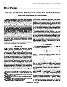
Practical experience shows that the numbers σi are good indicators of locality, because adding outliers to a good interpolant usually increases the error norm dramatically. Many of the σi can be expected to be small, and thus the threshold

σi < 2Mσ will be used to determine “good” points within the next splitting step, see Section 3.1.2, where Mσ is the median of all σi . This is illustrated for a data set by Figure 1: it represents, in base loglog scale, the sorted {σi } and the constant line relevant to the value of the threshold. 10 7

10 6

10 5

10 4

10 3

10 2

10 1

10 0

10 -1 10 0

10 1

10 2

10 3

Figure 1: Loglog: sorted {σi } and threshold

3.1.2 Splitting The set X g of points with good localization must now be split into J disjoint subsets of points that are close to each other. We assume that the inner boundaries of the subdomains are everywhere clearly determined by large values of σi . The implementation of this paper accomplishes the splitting by a variation of Kruskal’s algorithm [5] for calculating minimal spanning trees in graphs. The Kruskal algorithm sorts the edges by increasing weight and starts with an output graph that has no edges and no vertices. When running, it keeps a number of disconnected graphs as the output graph. It gradually adds edges with

3 IMPLEMENTATION

6

increasing weight that either connect two previously disconnected graphs or add an edge to an existing component or define a new connected component by that single edge. In the current implementation the edges that connect each xi with its n − 1 nearest neighbors are collected in an edge list. The edge list is sorted by increasing length of the edges and then, by n | X | comparisons, many repetitions of edges are removed, and these are all repetitions if any two different edges have different length. Then the thresholding of the {σi } by

σi < 2Mσ is executed, and it is known which points are good and which are bad. All edges with one or two bad end points are removed from the edge list with cost n | X |. After the spanning tree algorithm is run, the list of the points of each tree is intersected with itself to avoid eventual repetitions that are left. At the end, each connected component is associated to its tree in exactly one way. In rare cases, the splitting step may return only one tree, but these cases are detected and repaired easily.

3.2 Phase 2: Blow-up This is also an adaptive iterative process. It reduces the set X u := X \ ∪Jj=1 X jg of “unsure” data points gradually, moving points from X u to one of the nearest sets X jg . In order to deal with easy cases first, the points xi in X u are sorted by their locality quality such that points with better localization come first. We also g assume that for each point xi ∈ X u we know its distance to all sets X j , and we shall update this distance during the algorithm, when the sets X u and X jg change. g,0

We also use the distances to the sets X j that are the output of the localization g phase and serve as a start-up for the sets X j . In an outer loop we run over all points xi ∈ X u with decreasing quality of local approximation. In our implementation, this means increasing values of σi . The g inner loop runs over the m sets X j to which xi has shortest distance. In most cases, and in particular in R2 , it will suffice to take m = 2. The basic idea is to find the nearby set X jg of “good” points for which the addition of xi does least damage to the local approximation quality.

3 IMPLEMENTATION

7 g

Our implementation of the inner loop over m neighboring sets X j works as g,0

follows. In X j , the point y j with shortest distance to xi is picked, and its n nearest neighbors in X jg,0 are taken, forming a set Y jg . On this set, the data interpolant sgj is calculated, and then the number σ gj := ksgj kK measures the local approximation quality near the point y j if only “good” points are used. Then the “unsure” point xi is taken into account by forming a set Y ju of points consisting of xi and the up g to n − 1 nearest neigbors to xi from X j . On this set, the data interpolant suj is calculated, and the number σ uj := ksuj kK measures the local approximation quality if the “unsure” point xi is added to X jg . The inner loop ends by maintaining the minimum of quotients σ uj /σ gj over all nearby sets X jg checked by the loop. These quotients are used to indicate how much the local approximation quality would degrade if xi would be added to X jg . Note that this strategy maintains locality by focusing on “good” nearest neighbors of either xi or y j . By using the fixed sets g,0 g X j instead of the growing sets X j , the algorithm does not rely heavily on the newly added points. An illustration is attached to Example 1 in the next section; there the point y1 g and the sets X1 and Y1u associated to a point xi will be shown. After the inner loop, if the closest set to xi among all sets Xkg is X jg and σ uj /σ gj is less than σku /σkg for k 6= j, then xi is moved from X u to X jg . If the closest set to xi is X jg but if it is not true that σ uj /σ gj is less than σku /σkg for k 6= j, then xi remains “unsure”. The “unsure” points are those that seriously degrade the local approximation quality of all nearby sets of “good” points.

3.3 Phase 3: Final Assignment g

The assignment of a point xi ∈ X u to a set X j is done on the basis of how well the function value f (xi ) is predicted by u j (xi ). We loop over all points xi ∈ X u and first determine two sets X jg and Xkg to which xi has shortest distance. This is done in order to make sure that xi is not assigned to a far-away X jg . We then could add xi to X jg if | f (xi ) − u j (xi )| ≤ | f (xi ) − uk (xi )|, otherwise to Xkg , but in case that we have more than one unsure point, we want to make sure that under all unsure

4 EXAMPLES

8 g

g

points, xi fits better into X j than into Xk . Therefore we calculate d j (xi ) := | f (xi ) − u j (xi )| µ j := minu d j (xi ) xi ∈X

M j := maxu d j (xi ) D j (xi ) :=

xi ∈X d j (xi ) − µ j

Mj − µj

for all j and i beforehand, and assign xi to X jg if D j (xi ) ≤ Dk (xi ), otherwise to Xkg .

4 Examples Some test functions are considered now, each of which is smooth on J = 2 subdog g g g mains of Ω. The algorithm constructs X1 and X2 with X1 ∪ X2 = X . Concerning the error of approximation of u, we separate what happens away from the boundaries of Ω j from what happens globally on [0, 1]2. This is due to the fact that standard domain boundaries, even without any domain splittings, let the approximation quality decrease near the boundaries. To be more precise, let Ωsa f e be the union of the circles of radius q :=

min kxi − x j k2 ,

1≤i< j≤N

g

the separation distance of the data sites, centered at those points of X j , j = 1, 2 g such that the centered circles of radius 2q do not contain points of Xk with k 6= j. We then evaluate fe Lsa ∞ (u) := ku − f k∞,Ωsa f e ∩[0,1]2 and L∞ (u) := ku − f k∞,[0,1]2 . The chosen kernel for calculating the local kernel-based interpolants is the inverse multiquadric kernel φ (r) = (1 + 2r2 /δ 2 )−1/2 with parameter δ = 0.35. In all cases, N = 900 data locations are mildly scattered on a domain Ω that extends [0, 1]2 a little, with q = 0.04. We shall restrict to [0, 1]2 to evaluate the subapproximant, calculated by the basis in the Newton form. Such a basis is much more stable than the standard basis, see [6]. The error is computed on a grid with step 0.01.

4 EXAMPLES

9

Example 1. The function f1 (x, y) := log(| x − (0.2 sin(2π y) + 0.5) | +0.5), has a derivative discontinuity across the curve x = 0.2 sin(2π y) + 0.5. We get fe −5 −2 Lsa ∞ (u) = 1.6 · 10 , L∞ (u) = 6.0 · 10 .

For comparison, the errors of the global interpolant are fe ⋆ −1 ⋆ −1 Lsa ∞ (u ) = 1.1 · 10 , L∞ (u ) = 1.1 · 10 .

The classification turns out to be correct. 890 out of 900 data points are correctly classified as output of phase 3.2, and then phase 3.3 completes the classification. f f Figure 2 shows the points of X1 as dotted and those of X2 as crossed. The f points both dotted and circled of X1 , respectively the points both crossed and f circled of X2 , are the result of the splitting (Section 3.1.2), while the points dotted only, respectively crossed only, are those added by the blow-up phase (Section 3.2). The points squared are the result of the final assignment phase (Section 3.3). The true splitting line is traced too. The convention of the marker types will be used in the next examples as well. f The function u is defined as u1 where the subdomain Ω1 is determined and as f u2 on Ω2 . The actual error L∞ (u) = 6.0·10−2 is not much affected if we omit Phase 3 and and ignore the remaining 10 “unsure” points after the blow-up phase. A similar effect is observed for the other examples to follow. A zoomed area of Ω is considered in Figure 3. The details are related to an iteration of the blow-up phase, where the “unsure” point xi (both squared and g,0 starred) is currently examined. Points of X2 are shown as crosses. At the current g g,0 iteration, the dots are points inserted in X1 up to now, those belonging to X1 bold dotted, while the points inserted in X2g up to now are omitted in this illustration. g The points squared are those of Y1u , while the points as diamonds are those of Y1 . The point y1 is both written as diamond and star. Example 2. The function  f1 (x, y) if x 0.2 sin(2π y) + 0.5

4 EXAMPLES

10

has a discontinuity across the curve x = 0.2 sin(2π y) + 0.5. We get fe −5 −2 Lsa ∞ (u) = 1.6 · 10 , L∞ (u) = 6.0 · 10 . For comparison, the errors of the global interpolant are −1 ⋆ −1 fe ⋆ Lsa ∞ (u ) = 1.3 · 10 , L∞ (u ) = 1.3 · 10 .

The classification turns out to be correct. 888 out of 900 data points are classified correctly as output of phase 3.2, and phase 3.3 completes the classification for the f remaining 12 points. It might be that u j is more accurate on the safe zone, and also globally, Example 3. The function q f3 (x, y) := arctan(10 ( (x + 0.05)2 + (y + 0.05)2 − 0.7)) 3

(1)

is regular but has a steep gradient. Our algorithm yields fe −2 Lsa and L∞ (u) = 2.67 · 100, ∞ (u) = 9.0 · 10

while for the global interpolant we get fe ⋆ 0 ⋆ 0 Lsa ∞ (u ) = 2.31 · 10 , L∞ (u ) = 3.26 · 10 . f

f

f

f

Figure 4 shows the points of X1 as dotted and those of X2 as crossed; X1 and X2 stay at the opposite sides of the mid range line f (x, y) = 0 . Example 4. The function f4 (x, y) := ((x − 0.5)2 + (y − 0.5)2 )0.35 + 0.05 ∗ (x − 0.5)0+

(2)

has a jump on the line x = 0.5 and a derivative singularity on it at (0.5, 0.5). It has rather a steep gradient too. One data point close to the singularity is not classified correctly. We get fe −4 Lsa and L∞ (u) = 7.3 · 10−2, ∞ (u) = 9.9 · 10

while the global interpolant u⋆ has fe ⋆ −2 Lsa and L∞ (u⋆ ) = 8.5 · 10−2. ∞ (u ) = 1.5 · 10

4 EXAMPLES

11

Figure 5 shows the points of X1f as dotted and those of X2g as crossed. All examples show that the transition from a global to a properly segmented problem decreases the achievable error considerably. But the computational cost is serious, and it might be more efficient to implement a multiscale strategy that works on coarse data first, does the splitting of the domain coarsely, and then refines the solution on more data, without recalculating everything on the finer data. 1.2

1

0.8

0.6

0.4

0.2

0

-0.2 -0.2

0

0.2

0.4

0.6

0.8

1

Figure 2: Example 1: class 1 as dots, class 2 as crosses

1.2

REFERENCES

12

References [1] J.L. Bentley. Multidimensional binary search trees used for associative searching. Communications of the ACM, 18:509–517, 1975. [2] M.D. Buhmann. Radial Basis Functions, Theory and Implementations. Cambridge University Press, 2003. [3] N. Cristianini and J. Shawe-Taylor. An introduction to support vector machines and other kernel-based learning methods. Cambridge University Press, Cambridge, 2000. [4] G. Fasshauer and M. McCourt. Kernel-based Approximation Methods using MATLAB, volume 19 of Interdisciplinary Mathematical Sciences. World Scientific, Singapore, 2015. [5] J.B. Kruskal. On the shortest spanning subtree of a graph and the traveling salesman problem. Proceedings of the American Mathematical Society, 7:48–50, 1956. [6] St. Müller and R. Schaback. A Newton basis for kernel spaces. Journal of Approximation Theory, 161:645–655, 2009. doi:10.1016/j.jat.2008.10.014. [7] R. Schaback and H. Wendland. Kernel techniques: from machine learning to meshless methods. Acta Numerica, 15:543–639, 2006. [8] B. Schölkopf and A.J. Smola. Learning with Kernels. MIT Press, Cambridge, 2002. [9] J. Shawe-Taylor and N. Cristianini. Kernel Methods for Pattern Analysis. Cambridge University Press, 2004. [10] H. Wendland. Scattered Data Approximation. Cambridge University Press, 2005.

REFERENCES

13

0.9

0.8

0.7

0.6

0.5

0.4

0.2

0.3

0.4

0.5

0.6

Figure 3: Localized blow-up, zoomed in

0.7

REFERENCES

14

1.2

1

0.8

0.6

0.4

0.2

0

-0.2 -0.2

0

0.2

0.4

0.6

0.8

1

Figure 4: Example 3: class 1 as dots, class 2 as crosses

1.2

REFERENCES

15

1.2

1

0.8

0.6

0.4

0.2

0

-0.2 -0.2

0

0.2

0.4

0.6

0.8

1

Figure 5: Example 4: class 1 as dots, class 2 as crosses

1.2