large offshore wind farms concentrate a high wind power capacity at a single ...... ahead forecast that would minimize such criterion over the evaluation set.
Adaptive estimation in Markov-switching models for wind power short-term fluctuations Pierre Pinson Technical University of Denmark, Informatics and Mathematical Modelling, Kgs. Lyngby, Denmark
Henrik Madsen Technical University of Denmark, Informatics and Mathematical Modelling, Kgs. Lyngby, Denmark Abstract. Wind power production data averaged at a few-minute rate exhibit successive periods with fluctuations of smaller and larger magnitude, which cannot be explained (so far) by the evolution of some explanatory variable. This calls for the use of Markov-switching modelling approaches. Owing to long-term variations in the characteristics of the wind generation process, a Markov-switching autoregressive model with time-varying coefficients is introduced. Predictive densities can be analytically expressed as a finite mixture of conditional densities in each regime. Adaptive estimation of the model coefficients is based on recursive penalized maximum-likelihood. Its convergence and tracking abilities are assessed from simulations. The proposed models are then employed for modelling power fluctuations at two large offshore wind farms. They are evaluated on a 1-step ahead forecasting exercise. Its interest for better appraising the behaviour of power fluctuations is finally discussed.
1. Introduction Future developments of wind power installations are more likely to take place offshore, owing to space availability, less problems with local population acceptance, and more steady winds. This is especially the case for countries that already experience a high wind power penetration onshore, like Germany and Denmark for instance. This latter country hosts the two largest offshore wind farms worldwide: Nysted and Horns Rev, whose nominal capacities are of 165.5 and 160 MW, respectively. Today, each of these wind farms can supply alone 2% of the whole electricity consumption of Denmark (Sweet 2002). Such large offshore wind farms concentrate a high wind power capacity at a single location. Onshore, the same level of installed capacity is usually spread over an area of significant size, which yields a smoothing of power fluctuations (Focken et al. 2002). This smoothing effect is hardly present offshore, and thus the magnitude of power fluctuations may reach very significant levels. Characterizing and modelling the power fluctuations for the specific case of offshore wind farms is a current challenge (Akhmatov 2007, Hendersen et al. 2003), for better forecasting offshore wind generation, developing appropriate control strategies, or alternatively for simulating the combination of wind generation with storage or any form of backup generation. A discussion on these aspects is available in (Sørensen et al. 2007a). When inspecting offshore wind power production data averaged at a few-minute rate, one observes variations that are due to slower local atmospheric changes e.g. frontline passages and rain showers (Sørensen et al. 2007b). These meteorological phenomena add complexity to the modelling of wind power production, which is already non-linear and bounded
2
Pierre Pinson et al.
owing to the characteristics of the wind-to-power conversion function, the so-called power curve. Such succession of periods with power fluctuations of lower and larger magnitudes calls for the use of regime-switching models. Recently, Pinson et al. (2006) showed that for the case of the Nysted and Horns Rev wind farms, Markov-switching approaches, i.e. for which the regime sequence is not directly observable but is assumed to be a first-order Markov chain, were more suitable than regime-switching approaches relying on an observable process e.g. using Smooth Transition AutoRegressive (STAR) models. Though, a drawback of the Markov-switching approach described in (Pinson et al. 2006) is that model coefficients are not time-varying, while it is known that wind generation is a process with long-term variations due to e.g. changes in the wind farm environment, seasonality or climate change, see e.g. (Giebel et al. 2003). The main objective of the present paper is to introduce Markov-switching autoregressive models with time-varying coefficients, along with a suitable recursive estimation method, for application to the adaptive modelling of wind power fluctuations. The parameterization of the model coefficients employed here is inspired by those initially proposed in (Collings et al. 1994, Collings and Ryd´en 1998) and in (Holst et al. 1994). Adaptivity in time is achieved with exponential forgetting of past observations. In addition, the formulation of the objective function to be minimized at each time-step includes a regularization term that permits to increase the generalization ability of estimated models (in addition to improving numerical stability of the recursive estimation procedure). The motivation for introducing a recursive estimation method is to lower computational costs by updating estimates based on newly available observations only. In parallel, advantage is taken of the possibility to analytically formulate predictive densities from Markov-switching autoregressive models for associating one-step ahead forecasts with prediction intervals. Predictive densities are given as a mixture of conditional densities in each regime, the quantiles of which can be obtained by numerical integration methods. The paper is structured as following. A general formulation of the type of models considered, i.e. Markov-switching autoregressions with time-varying coefficients, is introduced in Section 2. The specific model parameterization employed is also described. Then, Section 3 focuses on the adaptive estimation of model coefficients, by first introducing the objective function to be minimized at each time-step, and then deriving an appropriate 3-step recursive estimation procedure. The issue of forecasting is dealt with in Section 4, by describing how one-step ahead point forecasts and quantile forecasts can be obtained, from a formulation of one-step ahead predictive densities. Simulations in Section 5 allow us to evaluate and highlight the properties of the proposed estimation method. Focus is given to the convergence and tracking ability of the method. Then, Markov-switching autoregression with time-varying coefficients is applied for modelling power fluctuations at offshore wind farms in Section 6. Data originates from both Nysted and Horns Rev wind farms, and consists in power averages with a 10-minute temporal resolution. The characteristics of the estimated models are discussed. Concluding remarks in Section 7 end the paper.
2. Markov-switching autoregression with time-varying coefficients Let {yt }, t = 1, . . . , n, be the time-series of measured power production over a period of n time steps. The power production value at a given time t is defined as the average power over the preceding time interval, i.e. between times t− 1 and t. For the modelling of offshore wind power fluctuations, the temporal resolution of relevant time-series ranges from 1 to 10 minutes. Hereafter, the notation yt may be used for denoting either the power production
Adaptive estimation in Markov-switching models for wind power short-term fluctuations
3
random variable at time t or the measured value. In parallel, consider {zt } a regime sequence taking a finite number of discrete values, zt ∈ {1, . . . , r}, ∀t. It is assumed that {yt } is an autoregressive process governed by the regime sequence {zt } in the following way, yt = with (z)
θt
xt
= =
(z)
�
(zt )
θt
(z)
�⊤
(zt )
xt + εt
∀t
,
(z)
[θt,0 θt,1 . . . θt,p ]⊤ ,
(1)
z = 1, . . . , r
(2)
⊤
(3)
[1 yt−1 yt−2 . . . yt−p ]
and where p is the order of the autoregressive process, chosen here to be the same in each regime for simplicity. However, the developed methodology could be extended for having different orders in each regime. The set of parameters for the Markov-switching model introduced above, denoted by Θt , is described here. The t-subscript is used for indicating that the autoregressive coefficients are time-dependent, though assumed to be (z) slowly varying. {εt } is a white noise process in regime z, i.e. a sequence of independent (z) random variables such that E[ε(z) ] = 0 and σt < ∞. Let us denote by η (z) the density function of the innovations in regime z, which we will refer to as a conditional density in the following. For simplicity, it is assumed that innovations in each regime are distributed (z) (z) Gaussian, εt ∼ N (0, σt ), ∀t, and thus !2 1 ε 1 , ∀z, t η (z) (ε; Θt ) = (z) √ exp − (4) 2 σt(z) σt 2π
with the t-subscript indicating that standard deviations of conditional densities are allowed to slowly change over time. In addition, it is assumed that the regime sequence {zt } follows a first order Markov chain on the finite space {1, . . . , r}: the regime at time k is determined from the regime at time k − 1 only, in a probabilistic manner, P [zk = j|zk−1 = i, zk−2 , . . . , z0 ] = P [zk = j|zk−1 = i],
∀i, j, k
(5)
All the probabilities governing switches from one regime to the others are gathered in the ij so-called transition matrix P(Θt ) = {pij t }i,j=1,...,r , for which the element pt represents the probability (given the model coefficients at time t, since transition probabilities are also allowed to slowly change over time) of being in regime j given that the previous regime was i, as formulated in (5). Some constraints need to be imposed on the transition probabilities. Firstly, by definition all the elements on a given row of the transition matrix must sum to 1, r X pij (6) t = 1, ∀i, t j=1
since the r regimes represent all possible states that can be reached at any time. Secondly, all the elements of the matrix are chosen to be positive: pij t ≥ 0, ∀i, j, t, in order to ensure ergodicity, which means that any regime can be reached eventually.
4
Pierre Pinson et al.
In order for constrainst (6) to be met at any time, the transition probabilities are parameterized on a unit sphere, as initially proposed in (Collings et al. 1994, Collings and Ryd´en � �2 ij i1 ir ⊤ 1998). Indeed, by having pij , and for each i, the vector si. det = [st . . . st ] t = st scribing a location on a r-dimensional sphere, we naturally have r X j=1
i. 2 pij t = ||st ||2 = 1,
∀i, t
(7)
For recursive estimation of coefficients in Markov-switching autoregression, Holst et al. (1994) argue that a more stable algorithm can be derived by considering the logarithms of the standard deviations of the model innovations, i.e. � � (z) (z) σ ˜t = ln σt , ∀z, t (8)
ij In a similar manner, it is also proposed here to consider the logit transform s˜ij t of the st coefficients in order to improve the numerical properties of the information matrix to be used in the recursive estimation scheme, ! sij ij t , ∀i, j, t (9) s˜t = ln 1 − sij t
which also translate to constraining the sij t coefficients to the [0, 1] interval. Finally, the set of coefficients allowing for full characterization of the Markov-switching autoregressive model at time t can be summarized as Θt =
�
where (z)
θt
(1) ⊤
θt
=
(r) ⊤
. . . θt
˜⊤ σ s⊤ t ˜
�⊤
h i⊤ (z) (z) (z) θt,0 θt,1 . . . θt,p ,
,
∀t
∀z, t
(10)
(11)
gives the autoregressive coefficients in regime j and at time t, while ˜t = σ
h i⊤ (1) (r) σ ˜t ... σ ˜t ,
∀t
(12)
corresponds to the natural logarithm of the standard deviations of conditional densities in all regimes at time t, and finally st =
�
⊤ ⊤ s˜1. . . . s˜r. t t
�⊤
,
∀t
(13)
is the vector of logit spherical coefficients summarizing the transition probabilities at that same time. 3. Adaptive estimation of the model coefficients There is a large number of papers in the literature dealing with recursive estimation in Hidden Markov Models (HMMs), see e.g. (Collings et al. 1994, Collings and Ryd´en 1998,
Adaptive estimation in Markov-switching models for wind power short-term fluctuations
5
Holst et al. 1994, LeGlang and Mevel 1997, Ryd´en 1997, Stiller and Radons 1999). Most of these estimation methods can be extended to the case of Markov-switching autoregressions. However, it is often considered that the underlying model is stationary and that recursive estimation is motivated by online application and reduction of computational costs only. In contrast here, the model coefficients are allowed to be slowly varying owing to the physical characteristics of the wind power generation process. This calls for the introduction of an adaptive estimation method permitting to track such long-term changes in the process characteristics. Hereafter, it is considered that observations are available up to the current point in time t, and hence that the size of the dataset grows as time increases. The time-dependent objective function to be minimized at each time step is introduced in a first stage, followed by the recursive procedure for updating the set of model coefficients as new observations become available. 3.1. Formulation of the time-dependent objective function If not seeking for adaptivity of model coefficients, their estimation can be performed (based on a dataset containing observations up to time t) by maximizing the likelihood of the observations given the model. Equivalently, given a chosen model structure, this translates to minimizing the negative log-likelihood of the observations given the set of model coefficients Θ, St (Θ) = − ln (P [y1 , y2 , . . . , yt | Θ]) (14) which can be rewritten as St (Θ) = − with
t X
ln (uk (Θ))
(15)
k=1
uk (Θ) = P [yk | yk−1 , . . . , y1 ; Θ]
(16)
In contrast, for the case of maximum-likelihood estimation for Markov-switching autoregression with time-varying coefficients, let us introduce the following time-dependent objective function to be minimized at time t ! t ν 1 X t−k (17) λ ln (uk (Θ)) + Θ⊤ Θ St (Θ) = − nλ 2 k=1
where λ is the forgetting factor, λ ∈ [0, 1[, allowing for exponential forgetting of past observations, and where 1 nλ = (18) 1−λ the effective number of observations is used for normalizing the negative log-likelihood part of the objective function. Note that (17) is a regularized version of what would be a usual maximum-likelihood objective function, with ν the regularization parameter. ν controls the balance between likelihood maximization and minimization of the norm of the model estimates. Such type of regularization is commonly known as Tikhonov regularization (Tikhonov and Arsenin 1977). It may allow to increase the generalization ability of the model when used for prediction. From a numerical point of view, it will permit to derive acceptable estimates even though the condition number of the information matrix used in
6
Pierre Pinson et al.
the recursive estimation procedure is pretty high. Theoretical and numerical properties of Tikhonov regularization are discussed in (Johansen 1997). ˆ t of the model coefficients at time t is finally defined as the set of The estimate Θ coefficient values which minimizes (17), i.e. ˆ t = arg min St (Θ) Θ
(19)
Θ
Note that to our knowledge, there is no literature on the properties of model coefficient estimates for Markov-switching autoregressions when the estimation is performed by minimizing (17). We do not aim in the present paper at performing the necessary theoretical developments. Instead, a simulation study in Section 5 will allow us to show the nice behaviour of the model estimates. 3.2. Recursive estimation Imagine being at time t, with the model fully specified by the estimate of model coefficients ˆ t−1 , and a newly available power measure yt . Our aim in the following is to describe the Θ ˆ t. procedure for updating the model coefficients and thus obtaining Θ Given the definition of the conditional probability uk in (16), i.e. as the likelihood of the observation yk given past observations and given the model coefficients (for a chosen model ˆ t−1 ) can be rewritten as structure), it is straightforward to see that at time t, ut (Θ ˆ t−1 ) = η ⊤ (εt ; Θ ˆ t−1 )P⊤ (Θ ˆ t−1 )ξ t−1 (Θ ˆ t−1 ) ut (Θ
(20)
ˆ t−1 ) In the above, εt is the vector of residuals in each regime at time t, thus yielding η(εt ; Θ the related values of conditional density functions (cf. (4)), given the model coefficients at ˆ t−1 ) is the vector of probabilities of being in such or such time t − 1. In addition, ξ t−1 (Θ regime at time t − 1, i.e. i h ˆ t−1 ) ˆ t−1 ) = ξ (1) (Θ ˆ t−1 ) ξ (2) (Θ ˆ t−1 ) . . . ξ (r) (Θ ξt−1 (Θ (21) t−1 t−1 t−1 given the observations up to that time, and given the most recent estimate of model coeffiˆ t−1 . In mathematical terms, this writes cients, that is, Θ i h (j) ˆ ˆ (22) ξt−1 (Θ t−1 ) = P zt−1 = j | yt−1 , yt−2 , . . . , y1 ; Θt−1
ˆ t−1 )ξ (Θ ˆ t−1 ) the forecast issued at time t − 1 of being in such or such then making P⊤ (Θ t−1 regime at time t. At this same time t, even if the set of true model coefficients Θt−1 were known, it would not be possible to readily say what the actual regime is. However, one can use statistical (j) inference for estimating the probability ξt of being in regime j at time t. This can indeed be achieved by applying the probabilistic inference filter initially introduced by Hamilton (1989), ⊤ ˆ ˆ ˆ ˆ t−1 ) = η(εt ; Θt−1 ) ⊗ P (Θt−1 )ξ t−1 (Θt−1 ) ξ t (Θ (23) ˆ t−1 )P⊤ (Θ ˆ t−1 )ξ t−1 (Θ ˆ t−1 ) η ⊤ (εt ; Θ where ⊗ denotes element-by-element multiplication. ξt will hence be referred to as the vector of filtered probabilities in the following.
Adaptive estimation in Markov-switching models for wind power short-term fluctuations
7
In order to derive the recursive estimation procedure, the method employed is based on ˆ t as a function of the previous using a Newton-Raphson step for obtaining the estimate Θ ˆ t−1 , see e.g. (Madsen 2007), estimate Θ ˆ ˆt = Θ ˆ t−1 − ∇Θ St (Θt−1 ) Θ ˆ t−1 ) ∇2Θ St (Θ
(24)
Few mathematical developments permit to obtain the formulation of the gradient of the objective function calculated at Θt−1 , ∇Θ St (Θt−1 ) = νΘt − λΘt−1 − (1 − λ)∇Θ ln(ut (Θt−1 ))
(25)
as well as its Hessian, � ∇2Θ St (Θt−1 ) = λ∇2Θ St−1 (Θt−1 ) + (1 − λ) µI − ∇2Θ ln(ut (Θt−1 ))
(26)
where I is an identity matrix of appropriate dimensions. In parallel, the gradient and Hessian of ln(ut (Θt−1 )) in (25) and (26) write ∇Θ ln(ut (Θt−1 )) = ht = and ∇2Θ ln(ut (Θt−1 )) =
∇Θ ut (Θt−1 ) ut (Θt−1 )
(27)
∇2Θ ut (Θt−1 ) ∇Θ ut (Θt−1 ) (∇Θ ut (Θt−1 )) − ut (Θt−1 ) u2t (Θt−1 )
⊤
(28)
However, by making the assumption such that ut is (almost) linear in Θ when calculated at Θt−1 , which translates to ⊤
∇2Θ ut (Θt−1 ) ∇Θ ut (Θt−1 ) (∇Θ ut (Θt−1 )) ≪ ut (Θt−1 ) u2t (Θt−1 )
(29)
one then obtains the following approximation of the Hessian of ln(ut ) evaluated at Θt−1 ∇2Θ ln(ut (Θt−1 )) ≃ −
∇Θ ut (Θt−1 ) (∇Θ ut (Θt−1 )) u2t
⊤
= −ht h⊤ t
(30)
Note that such assumption is somewhat similar to that made when applying a recursive Expectation-Maximization (EM) algorithm such as that proposed in (Holst et al. 1994). The necessary steps for obtaining ht are gathered in the Appendix. If denoting by Rt the matrix corresponding to the Hessian of ln(ut ), the 2-step scheme at time t for updating the set of model coefficients can be summarized as � Rt = λRt−1 + (1 − λ) ht h⊤ (31) t + νI io h n � � ˆ t−1 + (1 − λ)R−1 ht ˆ t = πs I + νR−1 −1 I + λνR−1 Θ (32) Θ t t t where I is an identity matrix of appropriate dimensions, and πs a projection operator on the unit spheres defined by the si. vectors (i = 1, . . . , r). This projection hence concerns transition probabilities only and do not affect autoregressive and standard deviation coefficients. Note that this 2-step scheme is applied after having calculated the vector of filtered probabilities ξ t .
8
Pierre Pinson et al.
One clearly sees in (31)-(32) the effects of regularization. It consists of a constant loading on the diagonal of the inverse covariance matrix Rt to be inverted in (32), thus permitting to control its condition number. Then, the second equation for model coefficients includes a dampening of previous estimates before and after updating with new information. One clearly sees that, when ν = 0, (32) simplifies to the classical updating formula for model coefficients tracked with Recursive Least Squares (RLS) or Recursive Maximum Likelihood (RML) methods. For more details, see e.g. (Madsen 2007). For initializing the recursive procedure without any information on the process considered, one may use equal probabilities of being in the various states, set the autoregressive coefficients to zero, put a large load on the diagonal elements of the transition matrix (i.e. large probabilities of staying in the same regime), and have sufficiently large standard deviations of conditional densities in each regime so that conditional density values are not too close to zero while having poor knowledge of the process. In parallel, the inverse covariance matrix R0 can be initialized with a matrix of zeros. Then, for the first few steps of the recursive estimation procedure, only (31) is used for gaining information as long as Rt is not invertible. After that, (32) can be used for updating model coefficient estimates. 4. Point and density forecasting Denote by ft the density function of wind power values at time t. Given the chosen model structure and the set of true model coefficients Θt−1 estimated at time t − 1, the one-step ahead predictive density of wind generation fˆt|t−1 can easily be expressed as fˆt|t−1 (y) =
r X j=1
� � (j) (j) (j) ξˆt|t−1 ηt−1 y − θt−1 ⊤ xt ; Θt−1
(33)
(j) where ξˆt|t−1 is the one-step ahead forecast probability of being in regime j at time t. The vector ξˆt|t−1 containing such forecast for all regimes is given by
ξˆt|t−1 = P⊤ (Θt−1 )ξ t−1 (Θt−1 )
(34)
Since the true model coefficients are obviously not available, they are replaced in the above ˆ t−1 available at that point in time. equations by the estimate Θ Define yˆt|t−1 the one-step ahead point prediction of wind power as the conditional expectation of the random variable yt , given the information set available at time t − 1. yˆt|t−1 can then be derived from the predictive density definition of (33) as yˆt|t−1 =
r X
(j) ˆ (j) ⊤ ξˆt|t−1 θ t−1 xt
(35)
j=1
since the distributions of innovations in each regime are all centered. In parallel, following the definition of conditional densities in (4), the one-step ahead predictive density fˆt|t−1 consists of a mixture of Normal densities. This predictive density can hence be explicitly formulated, and quantile forecasts for given proportions calculated with numerical integration methods. Indeed, if denoting by Fˆt|t−1 the cumulative distribu(α) tion function related to the predictive density fˆt|t−1 , the quantile forecast qˆt|t−1 for a given proportion α is (α) (36) qˆt|t−1 = Fˆt|t−1 −1 (α)
Adaptive estimation in Markov-switching models for wind power short-term fluctuations
9
The calculation of quantiles for finite mixtures of Normal densities is discussed in (Rahman et al. 2006). Note that the method proposed here disregards the question of uncertainty in parameter estimation, since it gives the exact formulation of the one-step ahead predictive density fˆt|t−1 given the true parameters of the Markov-switching autoregressive model. Accounting for parameter estimation uncertainty for such type of model is a difficult task which, to our knowledge, has not been treated in the relevant literature. The fact that model coefficients are time-varying and the proposed estimation method recursive complicates this question even more. However, the use of bootstrap methods may be envisaged, as initially proposed in (Craig and Sendi 2002). And, concerning the recursive estimation issue, one may consider adapting the nonparametric block bootstrap method introduced in (Corradi and Swanson 2007) to the case of the models considered here. 5. Simulations In this section, simulations are used for evaluating the convergence and tracking abilities of the proposed estimation method for Markov-switching regression with time-varying coefficients. Simulations are based on time-series of 20.000 time steps, with 2 periods of 10.000 time steps that correspond to 2 different Markov-switching autoregressions with Gaussian conditional densities. Over both periods, Markov-switching autoregressions have 2 regimes. In the first period, the autoregressive processes are characterized by (1)
θt
(1)
= [7 − 0.7]⊤ , σt
(2) θt
= 0.5, t = 1, . . . , 10.000
(2) σt
⊤
= [1 0.2] ,
= 1,
t = 1, . . . , 10.000
and the switching probability is set to 0.15. Then over the second period, the autoregressive processes are defined with (1)
θt
(1)
= 0.4, t = 10.001, . . . , 20.000
(2) σt
= 1.2, t = 10.001, . . . , 20.000
= [5 − 0.2]⊤ , σt
(2) θt
= [0 0]⊤ ,
and the switching probability is set to 0.2. Even if simulated processes are stationary Markov-switching autoregressions in each period, the abrupt change in all model coefficients at the end of the first period is expected to make the tracking of changes difficult for the adaptive estimation method. Our aim here is to follow the estimation error through time, and to see the behaviour of the estimates after the abrupt change in values of the true model coefficients at the end of the first period. For that purpose, we simulate 200 times the 20.000 time-step process described above, and follow the mean and some quantiles of the distributions of the estimation error for each of the model coefficients. The estimation error for a given model coefficient is defined as the difference between the value of the true model coefficient and that of the estimate. The quantiles chosen are those with proportion 0.05, 0.25, 0.75 and 0.95. For each of these simulated processes, the model parameterization described in section 2 and the adaptive estimation method introduced in section 3 are employed. The Markovswitching autoregressive process is initialized with (1)
θ0
(2) θ0
(1)
= 0.9
(2) σ0
= 0.9
= [5 0]⊤ , σ0 ⊤
= [0 0] ,
10
Pierre Pinson et al.
and the initial switching probability is set to 0.3. The forgetting factor λ and regularization parameter ν are chosen arbitrarily since our aim is not to obtain an optimal fitting but more to study the behaviour of the model coefficient estimates. However, owing to the fact that the processes considered are stationary in each period, a high value of λ is preferred. These two parameters are set to λ = 0.999 and ν = 0.0005. Other values of these 2 parameters have been tried, yielding similar results in a qualitative sense. The evolution of estimation error distributions is depicted in Figure 1 for the autoregressive coefficients, in Figure 2 for the standard deviations of conditional densities in each regime, and in Figure 3 for the transition probabilities.
mean quant (0.95) quant (0.75) quant (0.25) quant (0.05)
3
error
2 1
0.4 0.2 0
0
−0.2
−1
−0.4
−2 0
−0.6 0.5
1
1.5
2
0
0.5
1
1.5
4
error
1
2 4
x 10
x 10
0.2
0.5
0.1
0
0 −0.1
−0.5
−0.2 −1 0
0.5
1
time steps
1.5
2 4
x 10
0
0.5
1
time steps
1.5
2 4
x 10
Figure 1. Evolution of the estimation error distributions for the autoregressive coefficients of the (1) (1) (2) Markov-switching autoregressive model (top left: θt,0 , top right: θt,1 , bottom left: θt,0 , bottom right: (2) θt,1 ). Distributions are summarized by their mean and their quantiles with proportions 0.05, 0.25, 0.75 and 0.95.
Over the first period, there is a rapid convergence of the model coefficient estimates towards the true model autoregressive coefficients, especially for the level terms. Then, even after the abrupt change in process characteristics, the model coefficients also converge towards the new true values. One notices that the distributions of estimation error are pretty sharp around the mean, even after the abrupt change in process characteristics. When focusing on the evolution of the estimates of standard deviations of conditional
Adaptive estimation in Markov-switching models for wind power short-term fluctuations
11
densities in both regime (Figure 2), one globally sees the same kind of behaviour of the estimates, that is, a good ability for convergence, as well as for adaptation to an abrupt change in the process characteristics. Note that here, one may think that true standard deviation values are pretty close for the 2 periods, but actually, this translates to a significant difference in related conditional densities. Over the second period, the standard deviation of the conditional density in the second regime is significantly overestimated over a large number of time steps, and the distributions have heavy tails. However, for the 200 simulations, these model estimates converge to values pretty close to those of the true model coefficients.
0.1 0
error
−0.1
mean quant (0.95) quant (0.75) quant (0.25) quant (0.05)
−0.2 −0.3 −0.4 −0.5 0
0.2
0.4
0.6
0.8
1
1.2
1.4
1.6
1.8
2 4
x 10
0.4 0.3
error
0.2 0.1 0 −0.1 −0.2 −0.3 0
0.2
0.4
0.6
0.8
1
time steps
1.2
1.4
1.6
1.8
2 4
x 10
Figure 2. Evolution of the estimation error distributions for the standard deviations of conditional (1) (2) densities in each regime (top: σt , bottom: σt ). Distributions are summarized by their mean and their quantiles with proportions 0.05, 0.25, 0.75 and 0.95.
The transition probabilities are initialized to values that are far from the true ones. In addition, the true transition probabilities do not stay the same over the whole simulation period: there is a slight change from a switching probability of 0.15 to 0.2 when going from the first to the second period. It is known that transition probabilities are the most difficult coefficients to estimates in Markov-switching autoregressions (Holst et al. 1994). Note that due to the property such that transition probabilities on a given row of Pt sum to 1, the 21 12 22 estimation error in p11 t (respectively pt ) is the opposite of that in pt (respectively pt ).
12
Pierre Pinson et al.
This makes that the two plots on the right side of Figure 3 are the symmetric (with respect to the line y = 0) of those on the left side.
0.1 mean quant (0.95) quant (0.75) quant (0.25) quant (0.05)
0.15
error
0.1 0.05
0.05 0 −0.05
0 −0.1 −0.05 −0.15 −0.1 0
0.5
1
1.5
2
0
0.5
1
1.5
4
2 4
x 10
x 10
0.3
0.1
0.2
error
0 0.1 −0.1 0 −0.2 −0.1 0
0.5
1
time steps
1.5
2 4
x 10
0
0.5
1
time steps
1.5
2 4
x 10
Figure 3. Evolution of the estimation error distributions for the transition probabilities of the Markov12 21 22 switching autoregressive model (top left: p11 t , top right: pt , bottom left: pt , bottom right: pt ). Distributions are summarized by their mean and their quantiles with proportions 0.05, 0.25, 0.75 and 0.95.
Over the first period, there is a rapid and clear convergence of model estimates towards the true transition probabilities. Adaptation after the abrupt change in process characteristics is not as fast, especially for the second row of Pt . Indeed, for the case of p21 t and p22 t , the estimation error increases for 2500 time steps before the path towards convergence (2) is reinitiated. Such behaviour can also be noticed for the standard deviation σt of the conditional density in the second regime. These two comments may be linked, as intuitively, a larger standard deviation of the conditional density in a given regime makes that there is a higher probability of staying in the same regime. Distributions of estimation error have heavy tails for all transition probabilities, though their averages have a nice convergence towards 0 at the end of the dataset. Note that the (approximate) inverse covariance matrix used in the recursive estimation procedure has a large condition number, even if regularization is used. Therefore, some numerical issues may also be the reason why it is more difficult to estimate and track changes in standard deviations and transition probabilities
Adaptive estimation in Markov-switching models for wind power short-term fluctuations
13
coefficients. 6. Results on offshore wind power data In order to analyze the performance of the proposed Markov-switching autoregressions and related adaptive estimation method for the modelling of offshore wind power fluctuations, they are applied to real-world case studies. The exercise consists in one-step ahead forecasting of time-series of wind power production. Firstly, the data for the offshore wind farm is described. Then, the configuration of the various models and the setup used for estimation purposes are presented. Finally, a collection of results is shown and commented. 6.1. Case studies The two offshore wind farms are located at Horns Rev and Nysted, off the west coast of Jutland and off the south cost of Zealand in Denmark, respectively. The former has a nominal power of 160 MW, while that of the latter reaches 165.5 MW. The annual energy yield for each of these wind farms is around 600 GWh. Today, they represent the two largest offshore wind farms worldwide. For both wind farms, the original power measurement data consist of one-second measurements for each wind turbine. Focus is given to the total power output at Horns Rev and Nysted. For each wind farm , time series of power production are normalized by their rated capacity Pn . Hence, power values or error measures are all expressed in percentage of Pn . A sampling procedure has been developed in order to obtain time-series of 10-minute power averages. This averaging rate is selected so that the very fast fluctuations related to the turbulent nature of the wind disappear and reveal slower fluctuations at the minute scale. Because there may be some erroneous or suspicious data in the raw measurements, the sampling procedure has a threshold parameter τv , which corresponds to the minimum percentage of data that need to be considered as valid in a given time interval, so that the related power average is considered as valid too. The threshold chosen is τv = 75%. At Horns Rev, the available raw data are from 16th February 2005 to 25th January 2006. And, for Nysted, these data have been gathered for the period ranging from 1st January to 30th September 2005. 6.2. Model configuration and estimation setup From the averaged data, it is necessary to define periods that are used for training the statistical models and periods that are used for evaluating what the performance of these models may be in operational conditions. These two types of datasets are referred to as learning and testing sets. Sufficiently long periods without any invalid data are identified and permit to define these datasets. For both wind farms, the first 6000 data points are used as a training set, and the remainder for out-of-sample evaluation of the 1-step ahead forecast performance of the Markov-switching autoregressive models. These evaluation sets contain Nn = 20650 and Nh = 21350 data points for Nysted and Horns Rev, respectively. Over the learning period, a part of the data is used for one-fold cross validation (the last 2000 points) in order to select optimal values of the forgetting factor and regularization parameter. The autoregressive order of the Markov-switching models is arbitrarily set to p = 3, and the number of regimes to r = 3. For more information on cross validation, we refer to (Stone 1974). The error measure that is to be minimized over the cross validation
14
Pierre Pinson et al. Table 1. Forgetting factor λ and regularization parameter ν obtained from the cross validation procedure for the Nysted and Horns Rev wind farms. λ ν Nysted 0.998 0.005 Horns Rev 0.996 0.007
set is the Normalized Root Mean Square Error (NRMSE), since it is aimed at having 1-step ahead forecast that would minimize such criterion over the evaluation set. For all simulations, the autoregressive coefficients and standard deviations of conditional densities in each regime are initialized as (1)
θ0
(2) θ0 (3) θ0
(1)
= 0.15
(2) σ0 (3) σ0
= 0.15
= [0.2 0 0 0]⊤ , σ0 = [0.5 0 0 0]⊤ , ⊤
= [0.8 0 0 0] ,
= 0.15
while the initial matrix of transition probabilities is set to 0.8 0.2 0 P0 = 0.1 0.8 0.1 0 0.2 0.8
It is considered that the forgetting factor cannot be less than λ = 0.98, since lower values would correspond to an effective number of observations (cf. (18)) smaller than 50 data points. Such low value of the forgetting factor would then not allow for adaptation with respect to slow variations in the process characteristics, but would serve more for compensating for model mispecification. No restriction is imposed on the potential range of values for the regularization parameter ν. 6.3. Point forecasting results The results from the cross-validation procedure, i.e. the values of the forgetting factor λ and regularization parameter ν that minimize the 1-step ahead NRMSE over the validation set, are gathered in Table 1. In both cases, the forgetting factor takes value very close to 1, indicating that changes in process characteristics are indeed slow. The values in the Table correspond to number of effective observations of 500 and 250 for Nysted and Horns Rev, respectively, or seen differently to periods covering the last 3.5 and 1.75 days. Fast and abrupt changes in power fluctuations characteristics are dealt with thanks to the Markovswitching mechanism. In addition, regularization parameter values are not equal to zero, showing the benefits of the proposal. Note that one could actually increase this value even more if interested in dampening variations in model estimates, though this would affect forecasting performance. For evaluation of out-of-sample forecast accuracy, we follow the approach presented in (Madsen et al. 2005) for the evaluation of short-term wind power forecasts. Focus is given to the use of error measures such as NRMSE, Normalized Mean Absolute Error (NMAE), and Normalized bias (Nbias). In addition, forecasts from the proposed Markov-switching
Adaptive estimation in Markov-switching models for wind power short-term fluctuations
15
Table 2. One-step ahead forecast performance over the evaluation set for Nysted and Horns Rev. Results are both for persistence and Markov-switching models. Performance is summarized with Nbias, NMAE, and NRMSE criteria, given in percentage of the nominal capacity Pn of the wind farm considered. persistence Markov-switching model Nbias NMAE NRMSE Nbias NMAE NRMSE Nysted -0.0001 2.37 4.11 -0.0005 2.20 3.79 Horns Rev 0.0 2.71 5.06 -0.0004 2.70 4.96
autoregressive models are benchmarked against those obtained from persistence. Persistence is the most simple way of producing a forecast and is based on a random walk model. A 1-step ahead persistence forecast is equal the last power measure. Despite its apparent simplicity, this benchmark method is difficult to beat for look-ahead times such as that considered in the present paper. The forecast performance assessment over the evaluation set is summarized in Table 2. Predictions are unbiased whether issued from the persistence method of by using the Markov-switching approach. NMAE and NRMSE criteria have lower values when employing Markov-switching models. This is satisfactory as it was expected that predictions would be hardly better than those from persistence. The reduction in NRMSE and NMAE is higher for the Nysted wind farm than for the Horns Rev wind farm. In addition, the level of error is in general higher for the latter wind farm. This confirms the findings in (Pinson et al. 2006), where it is shown that the level of forecast performance, whatever the chosen approach, is higher at Nysted. The Horns Rev wind farm is located in the North Sea (while Nysted is in the Baltic sea, south of Zealand in Denmark). It may be more exposed to stronger fronts causing fluctuations with larger magnitude, and that are less predictable. An expected interest of the Markov-switching approach is that one can better appraise the characteristics of short-term fluctuations of wind generation offshore by studying the estimated model coefficients, standard deviations of conditional densities, as well as transition probabilities. Autoregressive coefficients may inform on how the persistent nature of power generation may evolve depending on the regime, while standard deviations of conditional densities may tell on the amplitude of wind power fluctuations depending on the regime. Finally, the transition probabilities may tell if such or such regime is more dominant, or if some fast transitions may be expected from certain regimes to the others. The set of model coefficients at the end of the evaluation set for Nysted can be summarized by the model autoregressive coefficients and related standard deviations of related conditional densities, (1)
θ Nn (2)
θ Nn (3)
θ Nn
= [0.0 1.361 − 0.351 − 0.019]⊤, = [0.013 1.508 − 0.778 0.244]⊤,
(1)
σNn = 0.0007 (2)
σNn = 0.041 (3)
= [−0.001 1.435 − 0.491 0.056]⊤, σNn = 0.011
while the final matrix of transition probabilities is 0.888 0.036 0.076 PNn = 0.027 0.842 0.131 0.051 0.075 0.874
In parallel for Horns Rev, the autoregressive coefficients and related standard deviations
16
Pierre Pinson et al.
are (1)
θ Nh (2)
θ Nh (3)
θ Nh
(1)
= [0.002 1.253 − 0.248 − 0.008]⊤, σNh = 0.023 = [0.022 1.178 − 0.3358 0.123]⊤, = [0.069 0.91 0.042 − 0.022]⊤,
(2)
σNh = 0.066 (3)
σNh = 0.005
while the final matrix of transition probabilities is 0.887 0.069 0.044 PNh = 0.222 0.710 0.068 0.173 0.138 0.689
For both wind farms, the first regime is dominant in the sense that it has the highest probability of staying in this same regime when it is reached. However, one could argue that the first regime is more dominant at Horns Rev, as the probabilities of staying in second and third regimes are lower, and as the probabilities of going back to first regime are higher. The dominant regimes have different characteristics for the two wind farms. At Nysted, it is the regime with the lower standard deviation of the conditional density, and thus the regime where fluctuations of smaller magnitude are to be expected. It is not the case at Horns Rev, as the dominant regime is that with the medium value of standard deviations of conditional densities. Such finding confirms the fact that power fluctuations seem to be of larger magnitude at Horns Rev than at Nysted. Let us study an arbitrarily chosen episode of power generation at the Horns Rev wind farm. For confidentiality reason, the dates defining beginning and end of this period cannot be given. The episode consists of 450 successive time-steps with power measurements and corresponding one-step ahead forecasts as obtained by the fitted Markov-switching autoregressive model. These 450 time steps represent a period of 75 hours. The time-series of power production over this period is shown in Figure 4, along with corresponding one-step ahead forecasts. In parallel, Figure 5 depicts the evolution of the filtered probabilities, i.e. the estimated probabilities of being in such or such regime at each time step. Finally, the evolution of the standard deviation of conditional densities in each regime is shown in Figure 6. First of all, it is important to notice that there is a clear difference between the three regimes in terms of magnitude of potential power fluctuations. There is a ratio 10 between the standard deviations of conditional densities between regime 2 and 3. In addition, these regimes are clearly separated, as there is a smooth evolution of the standard deviation parameters over the episode. If focusing on the power time-series of Figure 4, one observes successive periods with fluctuations of lower and larger magnitude. Then, by comparison with the evolution of filtered probabilities in Figure 5, one sees that periods with highly persistent behaviour of power generation are all associated with very high probability of being in the first regime. This is valid for time steps between 20 and 80 or between 380 and 450 for instance. This also shows that regimes are not obviously related to a certain level of power generation, as it would be the case if using e.g. Self-Exciting Transition AutoRegressive (SETAR) or Smooth Transition Auto-Regressive (STAR) models (Pinson et al. 2006). If looking again at the autoregressive coefficients in each regime given above for Horns Rev at the end of the evaluation period, one clearly sees that intercept coefficients are almost zero. While regime 1 appears to be the regime with low magnitude fluctuations, both regime 2 and 3 contribute to periods with larger ones. Studying obtained series of
Adaptive estimation in Markov-switching models for wind power short-term fluctuations
17
100 90
measures predictions
80
power [% Pn]
70 60 50 40 30 20 10 0 0
50
100
150
200
250
300
350
400
450
time step
Figure 4. Time-series of normalized power generation at Horns Rev (both measures and one-step ahead predictions) over an arbitrarily chosen episode. 1 0.9 0.8
probability
0.7 0.6
reg. 1 reg. 2 reg. 3
0.5 0.4 0.3 0.2 0.1 0 0
50
100
150
200
250
300
350
400
450
time step
Figure 5. Evolution of filtered probabilities given by the Markov-switching model over the same period. 6
5 regime 1 regime 2 regime 3
σ(z) [% Pn]
4
3
2
1
0
0
50
100
150
200
250
300
350
400
450
time step
Figure 6. Evolution of the standard deviation of conditional densities in the various regimes for the same episode.
18
Pierre Pinson et al.
filtered probabilities along with the evolution of some meteorological variables is expected to give useful information for better understanding meteorological phenomena that govern such behaviour. This would then permit to develop prediction methods taking advantage of additional explanatory variables.
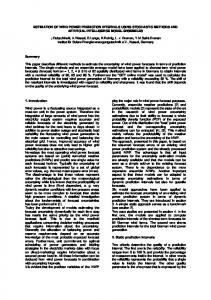
6.4. Interval forecasting results In a second stage, focus is given to the probabilistic information provided by the Markovswitching autoregressive models. Indeed, even if point predictions in the form of conditional expectations are expected to be relevant for power management purposes, the whole information on fluctuations will actually be given by prediction intervals giving the potential range of power production in the next time-step, with a given probability i.e. their nominal coverage rate. Therefore, the possibility of associating point predictions with central prediction intervals is considered here. Central prediction intervals are intervals that are centred in probability around the median. For instance, a central prediction interval with a nominal coverage rate of 80% has its bounds consisting of the quantile forecasts with nominal proportions 0.1 and 0.9. Therefore, for evaluating the reliability of generated interval forecasts, i.e. their probabilistic correctness, one has to verify the observed proportions of quantiles composing the bounds of intervals. For more information on the evaluation of probabilistic forecasts, and more particularly for the wind power application, we refer to (Gneiting et al. 2007, Pinson et al. 2007). Prediction intervals are generated over the evaluation set for both Horns Rev and Nysted. The nominal coverage of these intervals range from 10% to 90%, with a 10% increment. This translates to numerically calculating 18 quantiles of the predictive densities obtained from (33). The observed coverage for these various prediction intervals are gathered in Table 3. The agreement between nominal coverage rates and observed ones is good, with deviations from perfect reliability less than 2%. However as explained above, this evaluation has to be carried further by looking at the observed proportions of related quantile forecasts, in order to verify that intervals are indeed properly centred. Such evaluation is performed in Figure 7 by the use of reliability diagrams, which gives the observed proportions of the quantiles against the nominal ones. The closer to the diagonal the better. For both wind farms, the reliability curve lies below the diagonal, indicating that all quantiles are underestimated (in probability). This underestimation is more significant for the central part of predictive densities. Note that for operational applications one would be mainly interested in using prediction intervals with high nominal coverage rates, say larger than 80%, thus corresponding to quantile forecasts that are more reliable in the present evaluation. It seems that the Gaussian assumption for conditional densities allows to have predictive densities (in the form of Normal mixtures) that appropriately capture the shape of the tails of predictive distributions, but not their central parts. Using nonparametric density estimation in each regime may allow to correct for that. Finally, Figure 8 depicts the same episode with power measures and corresponding onestep ahead point prediction that than shown in Figure 4 for the Horns Rev wind farm, except that here point predictions are associated with prediction intervals with a nominal coverage rate of 90%. Prediction intervals with such nominal coverage rate are the most relevant for operational applications, and they have been found to be the most reliable in practice. The size of the prediction intervals obviously varies during this 450 time-step period, with their size directly influenced by forecasts of filtered probabilities and standard deviations of conditional densities in each regime (cf. (33)). In addition, prediction intervals are not
Adaptive estimation in Markov-switching models for wind power short-term fluctuations
19
Table 3. Empirical coverage of the interval forecasts produced from the Markov-switching autoregressive models for Horns Rev and Nysted. nom. cov. [%] obs. cov. Horns Rev [%] obs. cov. Nysted [%] 10 10.09 10.38 20 21.23 19.55 30 31.48 28.69 40 41.67 38.16 50 51.36 48.59 60 61.39 59.18 70 70.45 69.59 80 79.84 79.92 90 89.59 90.92
1 ideal Horns Rev Nysted
0.9
observed proportions
0.8 0.7 0.6 0.5 0.4 0.3 0.2 0.1 0
0
0.1
0.2
0.3
0.4
0.5
0.6
0.7
0.8
0.9
1
nominal proportions
Figure 7. Reliability evaluation of quantile forecasts obtained from the Markov-switching autoregressive models for both Horns Rev and Nysted. Such reliability diagram compare nominal and observed quantile proportions.
symmetric, as even if conditional densities are assumed to be Gaussian in each regime, the resulting one-step ahead predictive densities are clearly not. In this episode, prediction intervals are wider during periods with power fluctuations of larger magnitude. Even though point predictions may be less accurate (in a mean square sense) during these periods of larger fluctuations, Markov-switching autoregressive models can provide this valuable information about their potential magnitude. 7. Conclusions An appealing approach to the modelling of short-term wind power fluctuations, based on Markov-switching autoregressive models, has been introduced. Such an approach can be
20
Pierre Pinson et al.
100 0
measures predictions quant. forecasts (0.05) quant. forecasts (0.95)
90 80
power [% Pn]
70 60 50 40 30 20 10 0 0
50
100
150
200
250
300
350
400
450
time step
Figure 8. Time-series of normalized power generation at Horns Rev (both measures and one-step ahead predictions) over an arbitrarily chosen episode, accompanied with prediction intervals with a nominal coverage of 90%.
employed for simulation or forecasting purposes. Markov-switching autoregressive models have been generalized here so that they are allowed to have time-varying coefficients, though slowly varying, in order to follow the long-term variations in the wind generation process characteristics. An appropriate estimation method using recursive penalized maximum likelihood, where penalization consists of Tikhonov regularization, has been introduced. The proposal for including a regularization term comes from the aim of application to noisy wind power data, for which the use of non-regularized estimation may result in ill-conditioned numerical problems. The convergence and tracking abilities of the method have been shown from simulations. Then, Markov-switching autoregressive models have been employed for characterizing the 10-minute power fluctuations at Horns Rev and Nysted, the two largest offshore wind farms worldwide. The models and related estimation method have been evaluated on a one-step ahead forecasting exercise, with persistence as a benchmark. For both wind farms, the forecast accuracy of the proposed approach is higher than that of persistence, with the additional benefit of informing on the characteristics of such fluctuations. Indeed, it has been possible to identify regimes with different autoregressive behaviours, and more importantly with different variances in conditional densities. This shows the ability of the proposed approach to characterize periods with lower or larger magnitudes of power fluctuations. In the future, the series of state sequences may be compared with the time-series of some meteorological variables over the same period, in order to reveal if power fluctuations characteristics can indeed be explained by these meteorological variables. In addition to generating point predictions of wind generation, it has been shown that the interest of the approach proposed also lied in the possibility of associating prediction intervals or full predictive densities to point predictions. Indeed when focusing on power fluctuations, even if point predictions give useful information, one is mainly interested in the magnitude of potential deviations from these point predictions. It has been shown that for
Adaptive estimation in Markov-switching models for wind power short-term fluctuations
21
large nominal coverage rates (which are the most appropriate for operational applications) the reliability of prediction intervals was more acceptable than for low nominal coverage rates. It is known that for the wind generation process, noise distributions are not Gaussian, and that the shape of these distributions is influenced by the level of some explanatory variables (Pinson 2006). Therefore, in order to better shape predictive densities, the Gaussian assumption should be relaxed in the future. Nonparametric density estimation may be achieved with kernel density estimators, as in e.g. (Dorea and Zhao 2002), though this may introduce some problems in a recursive maximum likelihood estimation framework e.g. multimodality of conditional densities. One-step ahead predictive densities of power generation have been explicitly formulated. Such densities consist of finite mixtures of conditional densities in each regime. However, it has been explained that the issue of parameter uncertainty was not considered, and that this may also affect the quality of derived conditional densities, especially in an adaptive estimation framework where the quality of parameter estimation may also vary with time. Novel approaches accounting for such parameter uncertainty should hence be proposed. The derivation of analytical formula might be difficult. In contrast, one may think of employing nonparametric block bootstrap techniques similar to that proposed in (Corradi and Swanson 2007). This will be the focus of further research. Acknowledgments The results presented have been generated as a part of the project ‘Power Fluctuations in Large Offshore Wind Farms’ sponsored by the Danish Public Service Obligation (PSO) fund (PSO 105622 / FU 4104), which is hereby greatly acknowledged. DONG Energy Generation A/S and Vattenfall Danmark A/S are also acknowledged for providing the wind power data for the Nysted and Horns Rev offshore wind farms. Finally, the authors would like to acknowledge Tobias Ryd´en for fruitful discussions. References Akhmatov V. (2007) Influence of wind direction on intense power fluctuations in large offshore windfarms in the North Sea. Wind Eng., 31, 59-64. Collings I.B., Krishnamurthy V. and Moore J.B. (1994) On-line identification of hidden Markov models via prediction error techniques. IEEE T. Signal Proces., 42, 3535-3539. Collings I.B. and Ryd´en T. (1998) A new maximum likelihood gradient technique algorithm for on-line hidden Markov model identification. In Proc. IEEE Int. Conf. Acoust., Speech, Signal Processing, Seattle. Corradi V. and Swanson N.R. (2007) Nonparametric bootstrap procedures for predictive inference based on recursive estimation schemes. Int. Econ. Rev., 43, 67-109. Craig B.A. and Sendi P.P. (2002) Estimation of the transition matrix of a discrete-time Markov chain. Health Econ., 11, 33-42. Dorea C.C.Y. and Zhao L.C. (2002). Nonparametric density estimation in hidden Markov models. Stat. Infer. Stoch. Proc., 5, 55-64.
22
Pierre Pinson et al.
Focken U., Lange M., Monnich M., Waldl H.-P., Beyer H.-G. and Luig A. (2002) Short-term prediction of the aggregated power output of wind farms - A statistical analysis of the reduction of the prediction error by spatial smoothing effects. J. Wind Eng. Ind. Aerod., 90, 231-246. Giebel G., Kariniotakis G. and Brownsword R. (2003) The state of the art in short-term prediction of wind power - A literature overview. Position paper for the ANEMOS project, deliverable report D1.1, available online: http://www.anemos-project.eu. Gneiting T., Balabdaoui F. and Raftery A.E. (2007) Probabilistic forecasts, calibration and sharpness. J. R. Stat. Soc. B, 69, 243-268. Hamilton J.D. (1989) A new approach to the economic analysis of nonstationay time-series and business cycles. Econometrica, 57, 357-384. Hendersen A.R., Morgan C., Smith B., Sørensen H.C., Barthelmie R.J. and Boesmans B. (2003) Offshore wind energy in Europe - A review of the state-of-the-art. Wind Energy, 6, 35-52. Holst U., Lindgren G., Holst J. and Thuvesholmen M. (1994) Recursive estimation in switching autoregressions with a Markov regime. J. Time Ser. Anal., 15, 489-506. Johansen T.A. (1997) On Tikhonov regularization, bias and variance in nonlinear system identification. Automatica, 33, 441-446. Kim C.-J. (1994) Dynamic linear models with Markov-switching. J. Econ., 60, 1-22. LeGland F. and Mevel L. (1997) Recursive estimation in hidden Markov models. In Proc. IEEE CDC Conference, San Diego. Madsen H., Pinson P., Nielsen T.S., Nielsen H.Aa. and Kariniotakis G. (2005) Standardizing the performance evaluation of short-term wind power prediction models. Wind Eng., 29, 475-489. Madsen, H. (2007) Time-Series Analysis. London: Chapman & Hall. Pinson P. (2006) Estimation of the uncertainty in wind power forecasting. PhD Thesis, Ecole des Mines de Paris, France, available online: www.pastel.paristech.org. Pinson P., Christensen L.E.A, Madsen H., Sørensen P.E., Donovan M.H. and Jensen L.E. (2006) Regime-switching modelling of the fluctuations of offshore wind generation. J. Wind Eng. Ind. Aerod., submitted. Pinson P., Nielsen H.Aa., Møller J.K., Madsen H. and Kariniotakis G. (2007) Nonparametric probabilistic forecasts of wind power: required properties and evaluation. Wind Energy, 10, 497-516. Rahman M., Rahman R. and Pearson L.R. (2006) Quantiles for finite mixtures of Normal distributions. Int. J. Math. Educ. Sci. Tech., 37,352-357. Ryd´en T. (1997) On recursive estimation for hidden Markov models. Stoch. Proc. Appl., 66, 79-96.
Adaptive estimation in Markov-switching models for wind power short-term fluctuations
23
Stiller J.C. and Radons G. (1999) Online estimation of hidden Markov models. IEEE Signal Proc. Let., 6, 213-215. Sweet W. (2002) Reap the wild wind. IEEE Spectrum, 39, 34-39. Stone M. (1974) Cross-validation and assessment of statistical predictions (with discussion). J. R. Stat. Soc. B, 36, 111-147. Sørensen P.E., Cutululis N.A., Vigueras-Rodriguez A., Jensen L.E., Hjerrild J., Donovan M.H. and Madsen H. (2007) Power fluctuations from large wind farms. IEEE T. Pow. Syst., 22, 958-965. Sørensen P.E., Cutululis N.A., Vigueras-Rodriguez A., Madsen H., Pinson P., Jensen L.E., Hjerrild J. and Donovan M.H. (2007) Modelling of power fluctuations from large offshore wind farms. Wind Energy, in press. Tikhonov A.N. and Arsenin V.Y. (1977) Solutions of Ill-posed Problems. Washington: Wiscon.
Appendix: Derivatives of relevant variables In this Appendix are gathered some of the mathematical developments necessary for the application of the recursive estimation procedure at each time step t. More precisely, it gathers all necessary derivatives for obtaining ht as defined in (27). Mainly, it is necessary to derive ∇Θ ut and to give its value at Θt−1 . This is achieved by derivation of (20) as ∇Θ ut (Θt−1 ) =
⊤
(∇Θ η(εt ; Θt−1 )) P⊤ (Θt−1 )ξ t−1 (Θt−1 ) � + η ⊤ (εt ; Θt−1 ) ∇Θ P⊤ (Θt−1 ) ξ ⊤ t−1 (Θt−1 ) � ⊤ ⊤ + η (εt ; Θt−1 )P (Θt−1 ) ∇Θ ξ t−1 (Θt−1 )
(37)
In the above, the gradients of three different quantities need to be calculated, they correspond to the gradients of the conditional densities, of the transition probability matrix, and finally of the filtered probabilities. They are derived below. Gradient of the conditional densities η It is clear that η is independent of the s˜ij coefficients related to transition probabilities, and this whatever t. Therefore, for a given state j, ∇Θ η (j) (εt ; Θt−1 ) is composed by the vector of derivatives of η (j) with respect to the autoregressive coefficients and log-variances, calculated at εt , and by a vector of zeros of length r2 . (j) (j) The derivative of η (j) with respect to θi , calculated at εt given Θt−1 , writes (j)
∂θ(j) η (j) (εt ; Θt−1 ) = i
xt,j
(j) (j) ε η (j) (εt ; Θt−1 )δij (j) 2 t (σt−1 )
(38)
where xt,j is the j th element of xt , and where δij is an indicator variable, i.e. such that � 1, if i = j δij = (39) 0, otherwise
24
Pierre Pinson et al.
In parallel, the derivative of η (j) with respect to σ ˜ (j) , and calculated at εt , is similarly given by (j) 2 ε (j) (j) ∂σ˜ (j) η (j) (εt ; Θt−1 ) = t 2 − 1 η (j) (εt ; Θt−1 )δij (40) (j) σt−1 In practice, this means that it is only needed to compute r(p+ 1) derivatives for building ∇Θ η (j) (εt ; Θt−1 ) at each time step.
Gradient of the transition probability matrix P⊤ For the case of the transition probability matrix, things are just the other way around. That is, derivatives of P⊤ (Θt−1 ) with respect to autoregressive coefficients or to natural logarithms of standard deviations of conditional densities, so that it is only necessary to compute the r2 derivatives related to s˜ij coefficients. As a starting point, the derivative of P⊤ with respect to sij in the direction perpendicular to the constraint spherical surface defined by (7) is given in (Collings and Ryd´en 1998) and writes � ⊤ i. i. (41) ∂sij P⊤ (Θt−1 ) = 2sij t−1 ej − st−1 ⊗ st−1 ei with ej a vector of size r whose elements are zeros except for the j th , which equals 1. Then, by noticing that
and that one finally obtains
∂s˜ij P⊤ (Θt−1 ) = ∂sij P⊤ (Θt−1 )∂s˜ij sij t−1
(42)
ij ij ∂s˜ij sij t−1 = st−1 (1 − st−1 )
(43)
�2 � � ⊤ i. i. (1 − sij ∂s˜ij P⊤ (Θt−1 ) = 2 sij t−1 ) ej − st−1 ⊗ st−1 ei t−1
(44)
Gradient of the filtered probabilities ξ t−1 The probabilistic inference filter given in (23) permits to recursively estimate the vector of filtered probabilities. Therefore, by derivation of (23), one derives a similar filter permitting to recursively estimate ∇Θ ξt−1 from ∇Θ ξ t−2 , as well as ∇Θ P⊤ and ∇Θ η. First, note that one has ∇θ(1) ξ t−1 (Θt−1 ) .. . ∇ (j) ξ t−1 (Θt−1 ) θ .. ∇Θ ξ t−1 (Θt−1 ) = (45) . ∇ (r) ξ (Θt−1 ) t−1 θ ∇σ˜ ξ (Θt−1 ) t−1 ∇˜s ξ t−1 (Θt−1 ) The various elements composing ∇Θ ξ t−1 (Θt−1 ) are detailed below. Regarding derivatives with respect to the autoregressive parameters, one has (j)
∂θ(j) ξ t−1 (Θt−1 ) = τ t−1,i − i
ξt−1 (Θt−1 ) (j) | |τ ut−1 (Θt−1 ) t−1,i
(46)
Adaptive estimation in Markov-switching models for wind power short-term fluctuations
25
where (j)
τ t−1,i =
h� � � 1 (j) ∂θ(j) η (j) (εt−1 ; Θt−1 ) ej ⊗ P⊤ (Θt−1 )ξ t−2 (Θt−2 ) i ut−1 (Θt−1 ) � �i + η(εt−1 ; Θt−1 ) ⊗ P⊤ (Θt−1 )∂θ(j) ξ t−2 (Θt−2 ) (47) i
and |.| denotes the sum of the vector elements. In the above, ej is a unit vector as introduced in (41). ⊗ stands for the element-by-element multiplication. The derivatives with respect to the standard deviation of conditional densities in each regime are similar to those for the autoregressive parameters given in (46)-(47), that is, (j)
∂σ˜ (j) ξ t−1 (Θt−1 ) = χt−1 −
ξ t−1 (Θt−1 ) (j) |χ | ut−1 (Θt−1 ) t−1
(48)
where (j)
χt−1 =
h� � � 1 (j) ∂σ˜ (j) η(εt−1 ; Θt−1 ) ej ⊗ P⊤ (Θt−1 )ξ t−2 (Θt−2 ) ut−1 (Θt−1 ) �i + η(εt−1 ; Θt−1 ) ⊗ P⊤ (Θt−1 )∂σ˜ (j) ξ t−2 (Θt−2 )
(49)
In a similar manner, one can obtain the derivatives with respect to the s˜ij parameters calculated at Θt−1 . They are given by ∂s˜ij ξ t−1 (Θt−1 ) = ψ ij t−1 −
ξ t−1 (Θt−1 ) ij |ψ | ut−1 (Θt−1 ) t−1
(50)
where ψ ij t−1 = +
� h � 1 η(εt ; Θt−1 ) ∂s˜ij P⊤ (Θt−1 ) ξ t−2 (Θt−2 ) t−1 ut−1 (Θt−1 ) i ⊤ η(εt ; Θt−1 )P (Θt−1 )∂s˜ij ξt−2 (Θt−2 )
(51)