Consider an adaptive FIR filter with input Щn. The estima- tion error, at time .... the art in robust adaptive algorithms: NSLMP wn·Ð
. = wn. 1 u p p +. ( u) p/¾. NLMP.
ADAPTIVE FILTERING FOR NON-GAUSSIAN PROCESSES
Preben Kidmose Department of Mathematical Modelling, Section for Digital Signal Processing, Technical University of Denmark, Building 321, DK-2800 Lyngby, Denmark
ABSTRACT
1.2. Adaptive Filters Based on FLOM
A new stochastic gradient robust ltering method, based on a non-linear amplitude transformation, is proposed. The method requires no a priori knowledge of the characteristics of the input signals and it is insensitive to the signals distribution and to the stationarity of the signals. A simulation study, applying both synthetic and realworld signals, shows that the proposed method has overall better robustness performance, in terms of modeling error, compared with state-of-the-art robust ltering methods. A remarkable property of the proposed method is that it can handle double-talk in the acoustical echo-cancellation problem. 1. INTRODUCTION
Many signals encountered in practice are decidedly nonGaussian and the signals are only stationary up to an order less than 2. Recently [6] has investigated audio signals, and demonstrated the usefulness of the �-Stable distribution for modelling of noisy audio signals. In this work we consider robust adaptive algorithms. The objective is to design adaptive algorithms that are insensitive to the probability distribution and stationarity of the input signals. Consider an adaptive FIR lter with input un . The estimation error, at time n, of the lter is T
w un
(1)
where un is the input signal vector, w is the lter coeÆcient vector, and dn is the desired signal. Assume that dn and un are jointly stable processes of order �. The objective is to minimize the dispersion of the error, min jjdn en jj� . This objective turns out to be intractable, but fortunately proportional to the pth order moment for any 0 < p < �, [7]. So, an equivalent objective is J = E fjdn en jp g. There is no closed-form solution for the set of coeÆcients that minimize this objective; however the objective is convex for 1 � p � �, and so we may use a stochastic gradient method to solve for the coeÆcients. The class of stochastic gradient algorithms under consideration has the update wn+1
= wn
�h(en un )
h(eu) = (eu)hp=2i
as estimate of the gradient, [3]. Another subclass of normalized stochastic gradient algorithms, that has the form of Eq. 2, is proposed in [5]. The proposed lter update uses [hq (un )]i =
(2)
where h(�) is an estimate of the gradient E^ f@J=@ wg, based on the estimation error and the input.
jui;nPjq
1 sign(ui;n ) L ju jq m=1 i;n
for 1 � q < 1
(3)
where [hq (u)]i denotes the ith element of the vector valued function hq (u). This update, for � = 1 and for a valid q , corresponds to minimizing kwn+1 wn kp subject to dn T wn+1 un = 0. The relation between the norm, q , of the input signal vector, u, and the q -norm, of the coeÆcient vector update, kwn+1 wn kp , is 1=p + 1=q = 1, [5]. Thus, the update in Eq. 3 provides the minimum p-norm of the coeÆcient vector update. For q = 2 the algorithm is the classical NLMS algorithm. Recently [1] proposed a generalization to the NLMP with the update wn+1
1.1. Stochastic Gradient Algorithms
en = dn
A number of di�erent robust stochastic gradient algorithms, based on a fractional lower order moments (FLOM), has been proposed [1][2][3][5]. One of these is the Symmetric Least Mean P-norm (SLMP), that uses the symmetric norm
= wn
�
ehnai
h(q
un kun kqa qa + �
ai
1)
(4)
where, in the presence of an �-stable process, 0 < a � � 1 and 1 � q . For any real number v and p � 0, the convention v hpi = jv jp sign(v ) is used. The update is motivated by observing that it corresponds to a gradient descent adap� tation approach to the objective function J = E jen ja+1 . The update in Eq. 4 reduces to the NLMP update if a and q are chosen as p 1 and p=a. The update in equation 3 is a special case of Eq. 4 for a = 1 and � = 0 1.3. Median Orthogonality
If the median of the product, M (u1 u2 ), of two random variables u1 and u2 , is zero, then u1 and u2 are said to be median orthogonal, u1 ?MO u2 . For random variables with symmetric probability densities, independence is necessary and suÆcient for MO, however MO is necessary but not suÆcient for independence. The MO lter criterion, proposed in [2], is that the error should be MO to all elements of the input vector e ?MO u. This criterion extends the conventional orthogonality criterion without restricting the distribution of e and u.
2. A NEW ROBUST FILTERING METHOD
In this section we propose a conceptual di�erent approach to robust adaptive algorithms, that are based on a nonlinear amplitude transformation. The idea of the amplitude transformation is to ensure the existence of the second order moment.
The desired transformation, that transform a uniform distributed variable x~ into a variable y~, that follows the density g (y ), is y = G 1 (x), where G 1 (x) is the inverse function to the inde nite integral of g (y ). The transformation from a uniform distributed variable x~ into a variable y~ that follow the probability density p(y ) = g (y ), is depicted in Fig. 1. Thus, transformation between an arbitrary continuous
2.1. Density Transformation
The purpose of the non-linear amplitude transformation, is to transform the probability density of a signal. The proposed transformation, from an arbitrary unknown density to a desired density, is provided by a three-step procedure i Use the empirical density transformation, to obtain an uniform density. ii Transform with the inverse function to the inde nite integral of the desired density. iii Scale the transformed variable.
v
x
i
ii
y
iii
z
The scaling is necessary since all scale information is lost in the empirical density transformation. The objective of the scaling is to obtain kv kp = kz kp , for a suÆcient low p. 2.2. Empirical Transformation to Uniform Density
Let v~ be a random variable, and let v1 ; v2 ; : : : ; vN be N observations of the variable. An empirical transformation from the unknown arbitrary probability density random variable, v~, to the variable x~ with uniform density, can be done by sorting the observations. Sort the N observations, by the index m, such that v�;1 � v�;2 � � � � � vn;m � � � � � v�;N . The variable x~ is forced to follow the uniform density
p(x) =
�
1 2
0
r if if
jx aj � r jx aj > r
by assigning xn the value
r
p(x) r
x
x p(y)
y
Figure 1: Density transformation from an uniform probability density, p(x), to a probability density, p(y), by the function g(x). probability density to or from an uniform probability density, is given by the probability distribution function or the inverse probability distribution function respectively. 2.4. Stochastic Gradient Adaptive Filter Based on non-linear Transformation
The idea of the non-linear amplitude transformation, is to make a density transformation, that ensures the existence of the second order moment. We propose to use a transformation, g (�), that transform an arbitrary density into a Normal distribution. If the estimation error, en , and the input signal vector, un , is transformed into a Normal distributions by the�function ge (�) and gu (�), then the objective E jg (dn en )j2 makes sense. The structure of the adaptive algorithm is depicted in Fig. 2. The proposed amplitude transformation is sign con-
xn = (2m Nr)=N + a where m is the index that corresponds to the nth observation of v . The transformation is non-parametric and can be interpreted as the inverse cumulated histogram. The transformation, independent of the observations, result in an variable with uniform density. For variables with median equal to zero the transformation is sign conserving, and for symmetric densities the transformation is an odd function. Dependencies between variables are conserved. 2.3. Deterministic Density Transformation
The probability density of a random variable x~ is denoted p(x). The relation between the probability density for the random variable x~ and y~, is determined by the fundamental law of probability, p(y )dy = p(x)dx. Consider a transformation of the random variable x~, following the probability density p(x), to a new variable y~, following the probability density p(y ). Suppose that x~ follow a uniform distribution, and let g (y ) be a positive function with integral equal 1.
g(x)
P
h
u
e
P
w
gu
v
NLMS
ge
Figure 2: Adaptive lter based on a non-linear transformation of the estimation error.
serving, and that ensures that gu (u) ge (e) is an ascending direction for the objective function. A straightforward update equation, on the form of Eq. 2, is wn+1
= wn
�gu (un ) ge (en )
(5)
The median orthogonality (MO) criterion proposed in [2] apply to this update. The algorithm will have a stability point where e?MO u because the integral of the even density function and the odd g (�) is zero.
3. SIMULATIONS
0
The setup used for evaluation is depicted in Fig. 2, where h is an 10th order low pass lter. The proposed algorithm is compared to 3 other algorithms, that represents state of the art in robust adaptive algorithms: = wn
�
kukpp + a
NLMP
wn+1
= wn
�
kukpp + a e
Ayd�ins method
wn+1
= wn
�
1
h(q u
hp 1i u
ai
1)
hai
e kukqa qa + �
3.1. Simulation with synthetic signals
The synthetic signals are modeled as sequences of independent symmetric �-stable distributed random variables. The characteristic function for the random variable is given by �(t) = exp( jtj� ). The simulation of the signals are based on the method proposed in [4],[7]. The adaptation constants used in the simulation study, are listed in Table 1. Obviously these constants have considerably in uence on the characteristics of the algorithms. The constants are chosen such that all the algorithms are robust and stable in the wide range of signals under consideration in this simulation study. Note that, in the adAdaptation constants � = :01, p = q = 1:1, a = �v � = :01, p = :9�v , a = 10 6 � = :01, p = :9�v , a = 10 6 � = :05, N = 120
−20 −25 Aydins method NSLMP NLMP Proposed method
−30
0
1000
2000
3000
4000 5000 6000 number of iteration
7000
8000
9000
10000
Figure 3: Modeling error convergence for �u = �v = 1 and
u = v = 1. Mean over 10 Monte Carlo runs. 0
The performance of the algorithms are evaluated � as the modeling error 10 � log10 (w h)T (w h)=(hT h) .
Algorithm Ayd�ins method NSLMP NLMP Proposed method
−15
−40
−5 Modelling error [dB]
wn+1
−10
−35
(eu)hp=2i
NSLMP
−10 −15 Aydins method NSLMP NLMP Proposed method
−20 −25 0
1000
2000
3000
4000 5000 6000 number of iteration
7000
8000
9000
10000
Figure 4: Modeling error convergence for �u = 2, �v = 1 and
u = v = 1. Mean over 10 Monte Carlo runs. In Fig. 5 the modeling error versus signal to interference dispersion ratio is depicted. The dispersion of the −10
1:1
Table 1: Adaptation constants used in the system identi cation simulation study with �-stable signals vantage of the algorithms used for comparison, the norms used in these algorithms are adjusted in accordance with the applied signals. Consider the case where the input signal, u, and the interference signal, v , are identical white Cauchy distributed signals. The convergence of the modeling error is depicted in Fig. 3. All the methods converge to about the same misadjustment level, but the proposed method has the lowest misadjustment. Ayd�ins method has slower convergence than the other algorithms. For the case where the source signal, u, is a white Gaussian signal, and the interfering signal, v , is white following a Cauchy distribution, the convergence of the modeling error is depicted in Fig. 4. Two important changes are observed: the misadjustment level is about 20 dB higher and the convergence speed is slower. The -ratio is not a suitable measure between variables of di�erent distributions, so even though the -ratio between the signals is still equal to one, the empirical SNR is very poor.
Aydins method NSLMP NLMP Proposed method
−20 Modelling error, [dB]
1
Modelling error [dB]
−5
−30 −40 −50 −60 −70 −80 −1 10
0
10
u = v
10
1
2
10
Figure 5: Modeling error versus signal to interference dispersion ratio, uv . Characteristic exponent �u = �v = 1. source signal is varied in the interval u = [0:1; 100], and for the interfering signal the dispersion is constant, v = 1. For low dispersion ratios the performance of the algorithms are much the same; for increasing dispersion ratio the algorithms has increasing performance, and the proposed method takes increasing advantages compared to the other algorithms. In Fig. 6 the modeling error versus the characteristic exponent is depicted. The methods used for comparison are almost independent of �, since in this simulation study the norm is adjusted in accordance with the applied signal. Even though the proposed method does not require any knowledge of the input signals distribution it outperforms all the algorithms used for comparison. This is a remarkably robustness characteristic.
Modelling error, [dB]
−35 −40 −45 −50 Aydins method NSLMP NLMP Proposed method
−55 −60 1
1.1
1.2
1.3
1.4
1.5
�
1.6
1.7
1.8
1.9
2
Figure 6: Modeling error versus the characteristic exponent, �. The dispersion is u = 1 and v = 0:1. Mean over 10 Monte
Carlo runs.
3.2. Simulation with speech signals
Consider the adaptive algorithms used for acoustical echo canceling. The setup is as depicted in Fig. 2 where v is the local speaker and u is the remote speaker. The acoustical path, modeled by the lter h, is the same 10th order lter as in the previous simulation study. The adaptation constants used in this example are listed in Table 2. For the NSLMP, NLMP and Ayd�ins method the p-norm and � are set to relative small values to obtain stability. The signals are speech Algorithm Ayd�ins method NSLMP NLMP Proposed method
Adaptation constants � = :01, p = q = 1:1, a = :1 � = :01, p = 1:44, a = 10 6 � = :01, p = 1:44, a = 10 6 � = :1 , N = 1000
Table 2: Adaptation constants used in the acoustical echo cancellation for speech signals
signals sampled at 8kHz. The input signals and the modeling error result of the simulation is shown in Fig. 7. The local speaker
Modelling error [dB]
remote speaker 0 −10 −20 −30 −40 −50 0
5000
10000
15000
Aydins method NSLMP NLMP Proposed method 20000 25000
samples
Figure 7: Modeling error, in acoustical echo-canceler in crosstalk environment, for the 4 methods.
simulation example contains several diÆculties: the signals are non-stationary and contains temporal correlation, the amplitude density is non-Gaussian, and the dispersion ratio
between the signals are strongly varying. It appears, from Fig. 7, that the proposed method has slower convergence but apart from that, considerably better performance compared with the other methods. In the intervals where the local speaker is active, which corresponds to a poor SNR, the algorithms, except for the proposed method, loss the tracking of the lter. For these methods a control strategy is necessary. Contrary to the methods used for comparison, the proposed method has the ability to handle double-talk situations and environments with high background noise levels. 4. CONCLUSION
A new robust adaptive ltering method, based on a nonlinear amplitude transformation, is proposed. The method is compared with state-of-the-art robust ltering methods and a simulation study with synthetic and real-world signals is carried out. The proposed method requires no a priori knowledge of the input signals, it is insensitive to the signals density and to the stationarity of the signals. The proposed method has an overall better robustness performance, compared with state-of-the-art methods. The method is computational more expensive than the algorithms used for comparison, but these methods require either the use of a low p-norm or the estimation of a valid p, in order to ensure stability. A remarkable byproduct is that the proposed amplitude transformation method can be used in a variety of situations for signal conditioning. 5. REFERENCES
[1] Gul Ayd�in, Orban Ar�ikan, and A. Enis C�etin. Robust Adaptive Filtering Algorithms for �-Stable Processes. IEEE transactions on Circuits and Systems - II, 46(2):198{202, February 1999. [2] John S. Bodenschatz and Chrysostomos L. Nikias. Recursive Local Orthogonal Filtering. IEEE Transactions on Signal Processing, 45(9):2293{2300, 1997. [3] John S. Bodenschatz and Chrysostomos L. Nikias. Symmetric Alpha-Stable Filter Theory. IEEE Transactions on Signal Processing, 45(9):2301{2306, 1997. [4] J. M. Chambers, C. L. Mallows, and B. W. Stuck. A method for simulating stable random variables. Journal of the American Statistical Association, 71(354):340{ 344, 1976. [5] Scott C. Douglas. A Family of Normalized LMS Algorithms. IEEE Signal Processing Letters, 1(3):49{51, March 1994. [6] Panayiotis G. Georgiou, Panagiotis Tsakalides, and Chris Kyriakakis. Alpha-Stable Modeling of Noise and Robust Time-Delay Estimation in the Presence of Impulsive Noise. IEEE Transactions on Multimedia, 1(3):291{301, September 1999. [7] Chrysostomos L. Nikias and Min Shao. Signal Processing with Alpha-Stable Distribution and Applications. Wiley, 1 edition, 1995.