Adaptive Fuzzy Crop Edge Detection Method

Benson, E.R., J.F. Reid, Q. Zhang and F.A.C. Pinto. “An Adaptive Fuzzy Crop Edge Detection Method for Machine Vision.” Presented at the 2000 Annual ASAE Meeting, Paper No. 001019. ASAE, 2950 Niles Rd., St. Joseph, MI 49085-9659 USA.

Paper No.

001019 UILU 2000-7017

AN ADAPTIVE FUZZY CROP EDGE DETECTION METHOD FOR MACHINE VISION E.R. BENSON1, J.F. REID2, Q. ZHANG3, AND F.A.C. PINTO4 1Graduate

Fellow, Department of Agricultural Engineering, University of Illinois at Urbana - Champaign, IL, USA. Department of Agricultural Engineering, University of Illinois at Urbana - Champaign, IL, USA. 3Assistant Professor, Department of Agricultural Engineering, University of Illinois at Urbana - Champaign, IL, USA. 4Professor, Departamento de Engenharia Agrícola, Universidade Federal de Viçosa, BRAZIL. 2Professor,

Written for Presentation at the 2000 Annual International Meeting Sponsored by ASAE Milwaukee, WI July 9 – 12, 2000 Summary: The paper details a machine vision algorithm developed for crop edge detection. The algorithm was developed for an automated harvest application. The harvester needed the location and parameterization of the cut / uncut boundary for guidance. This paper details the development of one portion of the algorithm, an adaptive fuzzy sequential linear regression routine. A sequential linear regression routine was used to parameterize the crop edge. An adaptive fuzzy logic routine evaluated the performance of the regression and determined regression convergence. A second fuzzy routine evaluated the resulting regression. The regression output interfaced into fuzzy vehicle controller. The algorithm reduced the required processing by 77.1% versus a fixed region of interest and 58.6% versus a peak vertical transition region of interest.

KEYWORDS: vehicle guidance, corn harvest, machine vision, fuzzy logic, sequential linear regression The author(s) is solely responsible for the content of this technical presentation. The technical presentation does not necessarily reflect the official position of ASAE, and its printing and distribution does not constitute an endorsement of views which may be expressed. Technical presentations are not subject to the formal peer review process by ASAE editorial committees; therefore, they are not to be presented as refereed publications. Quotations from this work should state that it is from a presentation made by (name of author) at the (listed) ASAE meeting. EXAMPLE – From Author’s Last Name, Initials. “Title of Presentation.” Presented at the Date and Title of meeting, Paper No. X. ASAE, 2950 Niles Rd., St. Joseph, MI 49085-9659 USA. For information about securing permission to reprint or reproduce a technical presentation, please address inquiries to ASAE. ASAE, 2950 Niles Rd., St. Joseph, MI 49085-9659 USA. Voice: 616.429.0300 FAX: 616.429.3852

1


INTRODUCTION Agriculture has changed significantly since the introduction of the moldboard plow. Electronics including yield monitors, hitch controllers and GPS have become commonplace on modern agricultural tractors. Agricultural vehicle guidance has been a focus of research since the 1940’s and 50’s (Richey, 1959). Early agricultural guidance relied on mechanical or electrical control mechanisms. The solutions were limited and ultimately, not widely adopted. Advances in computing technology have allowed increased computational processing on the vehicle. High accuracy posture sensors are now available to accurately provide the position and orientation of the vehicle. Machine vision is an attractive technology for agriculture, combining accuracy, speed and relatively low cost in a non-contact form. For the combine guidance project, machine vision was well matched to the limited control available on the vehicle. Machine vision algorithms, however, can be crop and scene specific. One of the keys to a successful machine vision system is to extract the features of interest from the image. Researchers have developed methodologies to extract the features of crop rows from an agricultural scene (Reid and Searcy, 1991). Generally, the algorithms previously developed assume that the camera was located above and roughly parallel to the camera orientation. For row crop guidance (for example, cultivation), the vehicle is aligned with the rows and the crop is shorter than tractor mounted camera. The situation changes when the camera is used to guide a combine. The features of interest are no longer multiple crop rows, but the edge between the cut and uncut crop.

Figure 1:

The camera locations are dictated by practical considerations (Figure 1). Head mounted cameras run an increased chance of damage and require addition winter storage care and concerns. Vehicle mounted cameras, in contrast, are less likely to be damaged. A single camera mounted above the cab could potentially see the entire cutting swath, but would force a compromise between field of view and resolution. Perspective shift would cause discrepancies between the indicated crop and ground coordinates. Hoffman, et al., (1996) developed an automated harvester (Demeter) for alfalfa and other field crops. In the Demeter project, cameras were installed on both sides of the cab. Multiple cameras could be installed on the side of the combine; the typical combine uses several different heads during the course of the season. Each time the head with is changed, the image sensor would have to be aligned

Several potential camera locations on the combine

2


and calibrated. While potentially possible, it was not considered feasible to require the average farmer to periodically recalibrate the. Head mounted cameras could be positioned to directly see the cut / uncut edge, eliminating the perspective shift. Since the head mounted camera would remain with the head, the camera would not need to be recalibrated each time the head was changed. Due to the difficulties associated with a single top mounted camera, a multiple camera approach was investigated. In the multiple camera system, cameras were installed on each end of the head. The head mounted cameras allowed the camera to directly see the cut / uncut crop edge without the perspective shift issues of a high mounted camera. The head-mounted camera, however, sees a drastically different image than the top mounted cameras. A new image processing methodology was required to deal with the change in scene parameters.

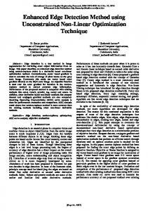
TYPICAL IMAGES A typical image from one of the head mounted Cohu 2100 series cameras is shown in Figure 2. The images contain several features of interest. The first feature of interest is the cut / uncut edge, marked by the letter A. The goal of the algorithm is to accurately parameterize the cut / uncut edge. To guide the vehicle, the lateral position of the cut / uncut edge needs to be controlled. The second feature of interest is the shadowed region (Region B). Many of the images contain shadows that obscure the actual cut / uncut edge. Since the goal is to track the cut / uncut edge, the stalk and leaves (Region C) are not relevant to processing. Most of the images contain both ground and sky, as represented by line D. Since the points above the line are not relevant for guidance, scene knowledge can be used to limit the processing region.

Figure 2:

A representative unprocessed image from one of the head mounted cameras. Features of interest include: A: Cut / Uncut edge B: Shadowed region C: Leaves and stalk D: Horizon

ALGORITHM DESCRIPTION A flow chart, shown in Figure 7 in Appendix A, details the basic structure of the combine guidance system. A second flow chart, shown in Figure 8 in Appendix B, shows the structure of the adaptive fuzzy crop edge detection algorithm. The algorithm is designed to extract the guidance signal from a suitable image. Secondary objectives included reducing the processing region and maintaining sufficient quality for guidance. Several assumptions were made during the development of the algorithm. Three major assumptions were: a) the wall effect, b) the camera directly viewed the cut / uncut

3


edge and c) the guidance objective was to control the lateral position of the cut / uncut edge. The “wall effect” can be seen in the representative image in Figure 4. It is not possible to see the inside rows from the outside row. The outermost row acts a wall, limiting the image scene. This creates an image in which only a single row is visible at any one time. In contrast, the typical tractor guidance algorithms utilize information from multiple rows to calculate a guidance signal. The cameras on the head were positioned to image the cut / uncut edge. Directly viewing the cut / uncut edge eliminated changes in the apparent ground location due to changed in the crop height. The third assumption influenced the selection of appropriate processing methods. The algorithm can be split into two portions: a row-based processing loop and a frame based processing component. The algorithm utilizes two fuzzy logic functions to a) determine when to stop process and b) to evaluate the image processing results. The algorithm is adaptive, adjusting the segmentation level, one of the fuzzy membership functions and the width of the region of interest (ROI) based on conditions. A goal of the algorithm was to reduce the size of the processed region to a minimum. The image was processed on a row-by-row basis from the bottom to the top. The upper portion of a typical harvest images contains sky and stalk, neither of which is relevant for determining the location of cut / uncut edge. A bottom to top processing routine processes the more important information first; the image processing can be terminated when performance reaches a satisfactory level. The key steps to the algorithm are image acquisition, extracting the image to memory, processing the image on a row-by-row basis, evaluating the quality of the results and adapting the width of the ROI for the next frame. Within the row processing loop, the key steps are segmentation, classification, sequential linear regression and fuzzy convergence estimation. Prior experience with the system indicated that the information towards the bottom of the image was more relevant than the information at the top of the image. This information was used to develop a fuzzy convergence evaluation scheme that weighted the vertical direction. Experience also showed that the crop images tended to be relatively noisy. The images tended to be relatively similar from frame to frame. Points that were far away from the previous regression line were highly likely to contain noise. A horizontal weighting formula was developed to reduce the impact of outliers.

IMAGE ACQUISITION: The algorithm was written to be largely hardware independent, however, the image acquisition commands depend on the specific frame grabber used. An ImageNation (Beaverton, CA) PXC-200 frame grabber was used during the course of the project. The native PXC-200 functions were used to initialize the frame grabber and grab the images. The algorithm was written with the capacity to handle multispectral images, but was implemented with monochrome image sources.

4


SEGMENTATION: An adaptive clustering algorithm was used to segment and classify the image. The image was segmented into two classes with an adaptive 2-class K-means clustering algorithm. The segmentation algorithm processes a given scan line point by point, calculating the RGB distance from each pixel to the mean class level (equation 1). The points are assigned to the class with the minimum RGB distance. The average class R, G and B values are calculated for each class at the end of the row and used to process the next row.

Di c =

(Ri − Rc )2 + (Bi − Bc )2 + (Gi − Gc )2

(1)

Where i is the pixel index, c is the class index, R is the red channel, B is the blue channel, G is the green channel and D is the RGB distance.

After classifying the points in a given scan line as cut or uncut, a heuristic algorithm detected the transitions between classes. A run length encoding algorithm reduced the individual transition points into a length (equation 2) and center location (equation 3). The run with the longest length for a given scan row and class (cut or uncut) was retained for future processing. The algorithm could be tuned to use either the cut or uncut class for processing.

l = (x ij − x(i −1)j )  x ij + x (i −1) j x j =  2 

(2)    

(3)

Where l is the distance between transitions, x is the column location of the transition, j is the row index and i is an index of transitions within the row.

SEQUENTIAL LINEAR REGRESSION:

2

Weight

A sequential linear regression algorithm was used to calculate the best-fit line for the transition points. The regression was performed on the center location of the longest run for a given scan line. In a ‘normal’ linear regression, the regression is calculated upon completion of the image processing. In a sequential linear regression, the regression parameters are updated during processing. The regression converges to a value; after convergence, additional points have little effect on the regression. The covariance matrix indicates the amount of scatter in the regression. The covariance, or scatter, can be used to determine when the regression results have satisfactorily converged. The

2.5

Linear

1.5

Sqrt 1/exp(X/100) 2 exp(-X/63)

1 0.5

0 0

100

200

300

400

Distance (pixels)

Figure 3:

5

Various sequential linear regression weighting factors.


regression can be stopped at any point after convergence with no effect on accuracy. One of the advantages of the sequential linear regression method was the weighting factor. The weighting factor can be set to unity, weighting all values equally, or can be used to bias towards certain results or regions. For combine guidance, information at the top of the image is further away and has less importance for the immediate guidance correction. False transitions, noise and outliers can cause problems for the regression. Two weighting formulas were developed for the sequential linear regression. The first weighting formula increased the weight of the points at the bottom of the image (Equation 4). The first formula was somewhat successful, but did not reduce the effect of noise. A second weighting formula was developed (Equation 5) that reduced the weight as the distance from the previous regression line increased. Several different weighting factors are shown in Figure 3. The second weighting formula decreases the weight of outliers and significantly improved the performance.

1   w = 1−   RowEnd 

(4)

    d −   (Im ageWidth)    10  

w = 2e d =| X j − X j |

(5)

X j = j * mi −1 + bi −1

(7)

(6)

Where w is the weight in the regression for a given transition, RowEnd is either the row indices for the peak vertical transition or the last processed line from the previous iteration, ImageWidth is the maximum width of the image in pixels, Xj is the characteristic point from above, d is the distance in pixels between the expected and actual transition, j is the row index, m is the linear regression slope from the previous image and b is the linear regression intercept from the previous image.

FUZZY EVALUATION: Fuzzy logic has been increasingly applied to a wide range of problems since introduced by Zadeh in 1965. Unlike Boolean logic, fuzzy logic is suited to evaluating subjective situations. For agriculture, the subjectivity of fuzzy logic is particularly appealing (Ribeiro, 1999, Wang, 1996, Zhang and Litchfield, 1991, 1994). Field conditions – weather, the position and intensity of the sun and dust, just to name a few – and crop conditions – size, shape, weed and pest pressure – combine to create a difficult situation for conventional evaluation methods.

Row Index Input Membership Functions Maximum Image Height - 50 Membership Function

Good

Bad

Transition End

Maximum Image Height

Row Location

Figure 4:

6

The adaptive fuzzy input membership function.


Fuzzy logic allows a problem to be represented as linguistic variables rather than crisply defined values. Fuzzy logic allows the developer to take advantage of a priori knowledge about the system to describe the relationship(s) between the input and output. In fuzzy logic, the range, or universe, of values is represented by U. A fuzzy set is defined in U and characterized by the membership function µF in the range [0, 1]. For any two fuzzy sets (S1, S2) in U, three basic operations can be defined: Intersection:

µ S1∩ S 2 = min{ µ s1(u), µ s 2 (u)}

Union:

µ S1∪ S 2 = max{ µ s1(u), µ s2 (u)}

Complement:

µ s1 = 1− µ s1

The fuzzy decision making process is based on a system of rules (rules base) that defines the mapping from the input to fuzzy classification and back again. An example (Figure 4) of a fuzzy rule would be: If (Row Location < TransitionEnd) then the fuzzy classification is “Good”. In the example above, the input is mapped into a single membership function, but in actual use, the membership function is typically mapped into portions of two different functions (continuing the example above, 0.3 Good and 0.7 Bad). The membership function is represented by the intersection operator shown above. A similar procedure is used during defuzzification to map from the fuzzy membership functions to a crisp value. Different methods, including center of gravity, have been posed for defuzzification. A generic fuzzy module was developed for the project. The fuzzy module operated on the assumption of independence between parameters. The fuzzy module membership functions could be static or changed during processing. For programming convenience, the fuzzy module was restricted to triangular and trapezoidal membership functions. The module used a center of gravity defuzzification approach. Fuzzy Convergence Evaluation: One of the objectives of the algorithm was to reduce the size of the processed region, allowing potential improvements in the processing speed. Experience with the sequential linear regression algorithm showed that the solution would typically converge to a result well before the entire image was processed. Processing additional points typically had little effect on the solution. Each additional scan line processed added a significant computational load to the image processing requirements. The slope and intercept covariance estimates from the sequential linear regression indicated the relative amount of scatter in the data. The covariance, or scatter, provided information on the regression convergence. The minimum acceptable slope and intercept covariance were determined from experience with the system. In addition to the scatter, an additional parameter was the vertical position in the image. The fewer the scan lines processed, the faster the algorithm. The relatively noisy images, however, placed a practical limitation on the minimum acceptable processing region.

7


In the interest of algorithm speed, as the size of the processed region increases, it becomes increasingly important to terminate processing. A three-input Fuzzy Convergence Evaluation model was developed for the system. The three inputs were: slope covariance, intercept covariance and row postion. The covariance membership functions were tuned to the system. The row position membership function was adaptive and changed based on size of the processing region from the previous frame. The row position term acted as a vertical weighting factor, allowing the importance of various portions of the image to be manipulated. Each of the three inputs utilized two trapezoidal fuzzy membership functions (Acceptable and Unacceptable). A single output was created using a center of gravity approach with two trapezoidal membership functions (Stop or Continue). The Fuzzy Convergence Evaluation module classes are shown in Figure 10 in Appendix C. The output from the fuzzy linear regression indicated when to stop processing the image. A counter was used to eliminate false positives on small data sets. If the covariances and the row index did not meet the predefined quality requirements, then the next line of the image was processed. If the inputs met the desired quality requirements, then the row-by-row image processing was halted and processing switched from row processing to overall frame processing. The line index upon convergence was recorded as the transition end. The row location membership function was adaptively tuned. An external specification file provided initial values or values in the event of an error. The transition end value was used to adapt the row index membership functions for the next image. The row end membership functions are shown in Figure 4. Although fuzzy logic was used to evaluate the regression, a fuzzy linear regression methodology was not used. Fuzzy linear regression is different from the staged sequential regression and fuzzy quality analysis methodology implemented. Redden and Woodall (1996) note that fuzzy linear regression algorithms can be extremely sensitive to outliers. The transition image was characterized by a large number of outliers; a fuzzy linear method would be ill suited to the problem at hand. The row-by-row image processing was halted when the fuzzy linear output indicated that the regression had reached predefined quality measures. Alternatives to the fuzzy linear quality module included peak vertical transition or a fixed vertical window position. The peak vertical transition methodology consisted of a ‘voting’ approach. Each time there was a transition between classes in the vertical direction, the value was recorded in a histogram. The row index corresponding to the largest histogram bin was the peak vertical transition. Calculating the histogram required analyzing each pixel in the image. The peak vertical transition was then used to restrict subsequent processing. The peak vertical transition method was initially implemented in the system, but was made unnecessary by the Fuzzy Convergence Evaluation module. Fuzzy Quality Evaluation: A second fuzzy logic module evaluated the results from the regression. The module was added due to harvest experience. The cameras were positioned above and to the side of the snap rolls. As the snap rolls grabbed the stalks, stalks would occasionally be forced in front of the camera. Grabbing an image as the stalk passed in front of the camera resulted in valid, but unreasonable results.

8


The range of acceptable slopes (0 to 180, with preferred regions within the ranges) and intercept (within the image) were defined based on experience with the sytem. Experience also indicated that the images remained relatively constant frame to frame. Large variations from one frame to the next were most likely due to leaves or other obstacles passing in front of the camera. Since the images tended to be similar frame to frame, the results from the previous image could be used in the event of a problem. A four-input fuzzy logic module was used to evaluate the output from the regression. The four inputs for the Fuzzy Quality Evaluation function were percent change in slope, percent change in intercept, processed slope and processed intercept value. The membership functions for the Fuzzy Quality Evaluation are shown in Figure 11 in Appendix D. As in the fuzzy linear quality module, trapezoidal membership functions and the center of gravity approach were used. The single output from the Fuzzy Quality Evaluation module indicated whether to accept the regression results or default to the result from the previous image.

ADAPTIVE REGION OF INTEREST: After completion of the Fuzzy Quality Evaluation module, an adaptive region of interest algorithm adjusted the width of the processed region. In this application, the ideal width of the processed region is a trade off between processing time and flexibility. A smaller processing window improves the processing time, at the expense of eliminating potentially useful information. The adaptive region of interest module adjusted the horizontal position of the processed region based on the regression results. The vertical size of the processed region was dictated by the Fuzzy Convergence Evaluation module. The adaptive region of interest algorithms is not covered in this paper.

PROCEDURE: The image processing algorithm described above was developed for combine harvester guidance. A Case 2188 Axial-Flow combine (Figure 5) was prepared for guidance use. The modifications relevant to the image processing included the installation of cameras on the sides of the Case 1083 8-row corn head and above the cab. Additional information on the overall system is available in Benson, et al. (2000). Several different cameras were used during the fall harvest; the cameras used for this study were Cohu 2100 series monochrome cameras equipped with 800 nm narrow band NIR filters.

Figure 5: The Case 2188 Combine research platform

Before the season began, several different camera locations were tried. For harvest, however, two camera locations (right and left side of the head) were used. The camera was mounted in an open-ended cage for protection. The camera underwent both translation and rotation as the head was raised and lowered in the field. The camera

9


was located approximately 2 m from the ground while harvesting. The camera configuration is shown in Figure 6. Initial algorithm development was done with video footage recorded during the fall 1999 harvest. The system was validated using late season corn. The baseline computer used for processing was a 266 MHz or higher Pentiumcompatible computer with an ImageNation PXC200 color frame grabber. The image processing software was written in C using the Microsoft Visual Studio. Figure 6:

The head mounted cameras

Three methods were compared: Full image processing, vertical transition image reduction and adaptive fuzzy linear regression. The same image sequence was used for all three methods. The processing methodologies were evaluated by comparing the image processing space for the same harvest sequence. Fifty-one images were processed and the relevant statistics were determined. The image processing was repeated three times for approximately the same section of video footage.

RESULTS The fuzzy sequential linear regression algorithm reduced the size of the processed region when compared to other methods. For the image sequence analyzed, full image processing required processing 476 lines. Adding the vertical transition allowed the processing to be reduced from 476 rows to 265.7 rows (σ = 49.4 rows). The adaptive fuzzy linear regression required 109.4 rows (σ = 40.0 rows). The differences between each of the three methods were statistically significant (Table 1). A representative processed image is shown in Figure 7. The vertical transition line is indicated on the image. The output from the fuzzy linear regression quality module was used to stop the image processing. The vertical transition line was clearly higher in the image than the height required for the regression. The additional image height increased the required image processing. From the

Vertical Transition Line

Regression Line

Class 1

Figure 7:

10

Class 2

A representative processed image


image, it can also be seen that less than 50% of the image was processed; a fixed region of interest (ROI) would be relatively inefficient. During validation, the image processing algorithm was used to guide the combine. The algorithm satisfactorily guided the combine through the corn. Table 1: Paired z-test for unequal mean and variance Z Value Fixed Peak Vertical Adaptive Fixed -52.70 -113.34 Peak Vertical -52.70 -30.42

CONCLUSIONS A machine vision algorithm was developed to determine the parameterization of a row of corn. The algorithm used sequential linear regression linked to a pair of fuzzy logic modules to determine the processing requirements and to improve the quality. The algorithm was evaluated using video recorded during harvest and validated in late season corn. The algorithm was compared to a fixed and a peak vertical transition height region of interest methods. The algorithm reduced the processing requirements by 77.2% and 58.6% respectively.

ACKNOWLEDGEMENTS The research presented was supported by CNH Global NV. Funding for Eric Benson was provided by a fellowship from the University of Illinois College of Agricultural, Consumer and Environmental Sciences. The authors would also like to thank the UIUC Crop Science and Agricultural Engineering Departments for providing corn to harvest and harvest support. The authors would also like to thank Birkey’s Farm Store in Urbana, IL for their assistance in preparing the guidance combine.

BIBLIOGRAPHY Benson, E.R., J.F. Reid, and Q. Zhang, 2000. “Development of an Automated Combine Guidance System.” ASAE Paper 003137. St. Joseph, MI. Redden, D.T., and W.H. Woodall, 1996. Further examination of fuzzy linear regression. Fuzzy Sets and Systems 79(2): 203 – 211. Reid, J., and S.W. Searcy, 1991. An algorithm for computer vision sensing of row crop guidance directrix. SAE Paper 911752. Warrendale, PA. Ribeiro, R.A. 1999. Fuzzy evaluation of the thermal quality of buildings. Computer-Aided Civil and Infrastructure Engineering, 14: 155-162. Richey, C.B. 1959. “Automatic Pilot” for farm tractors. Agricultural Engineering 40(2): 1959 78 – 79, 93. Hoffman, R., K. Fitzpatrick, M. Ollis, H. Pangels, T. Pilarski and A. Stentz, 1996. Demeter: an autonomous alfalfa harvesting system. ASAE Paper 963005. St. Joseph, MI. Wang, J. and V. Allada. 1996. Fuzzy logic approach for serviceability evaluation. Intelligent Engineering Systems through Artificial Neural Networks 1996(6): 1075-1080. Zadeh, L.A. 1965. Fuzzy Sets. Information and Control 8: 338-53.

11


Zhang, Q., and J.B. Litchfield. 1994. Knowledge representation in a grain drier fuzzy logic controller. J. agric. Engng Res. 57: 269-278. Zhang, Q., and J.B. Litchfield. 1991. Applying fuzzy mathematics to product development and comparison. Food Technology 1991: 108 – 115. Appendix A: Overall system flow chart

Figure 8:

Overall System Flow Chart

Appendix B: Algorithm flow chart

Figure 9:

Algorithm Flow Chart

12


Appendix C: Fuzzy Convergence Evaluation membership functions

Slope Input Membership Functions Membership Function

Good

Bad

0.001

0.20

Covariance Intercept Input Membership Functions Membership Function

Good

Bad

1E-6

5E-6 Covariance

Row Index Input Membership Functions Membership Function

Bad

Good

10

440* Row Location

*Note: The row location was adaptively tuned after the first iteration Output Membership Functions Membership Function Continue -1.2

Stop

-0.75

0.75 1.0

Output Value Figure 10:

Top: Slope input membership function Upper Middle: Intercept membership function Lower Middle: Row index membership function Bottom: Output membership 13 function


Appendix D: Fuzzy Quality Evaluation membership functions

Percent Change Slope Input Membership Functions Membership Function

Good 0

Bad 20

45

Percent Change Intercept Input Membership Functions

Really Bad

Good

60

0

Abs(Percent Change)

20

45

Really Bad 60

Abs(Percent Change) Intercept Input Membership Functions

Slope Input Membership Functions Membership Function

Bad

Bad Low 0 45

Good 60

120

Really Bad

High 135

0 10 20

Slope (degrees)

Really Bad

Good

300 320 340

Intercept

Output Membership Functions

Membership Function

Really Bad -3.5

-2.5

Bad

Good

-1.25 -0.85

0.75

1.0

Output Value Figure 11:

Top Left: Percent change in slope input membership function Top Right: Percent change in intercept input membership function Middle Left: Processed slope input membership function Middle Right: Processed intercept input membership function Bottom: Output membership function

14

Adaptive Fuzzy Crop Edge Detection Method

Adaptive Fuzzy Crop Edge Detection Method

Suggest Documents

An Adaptive Fuzzy Classifier Approach to Edge Detection in Latent ...

A FUZZY LOGIC BASED METHOD FOR EDGE DETECTION

An Improved NMS-Based Adaptive Edge Detection Method and Its ...

Enhanced Edge Detection Method using

Image Edge Detection with Fuzzy Classifier - CiteSeerX

Adaptive Ontology Construction Method for Crop Pest

Fuzzy Edge Detection by Fuzzy Categorization and Classification of ...

AN ADAPTIVE EDGE ELEMENT METHOD WITH

Adaptive Threshold Edge Detection Algorithm ... - Semantic Scholar

An Adaptive Edge Detection for Mycosis

An Adaptive Fuzzy k-Nearest Neighbor Method

Hybrid Adaptive Bionic Fuzzy Control Method

Adaptive Neuro-Fuzzy Modeling For Crop Yield Prediction - wseas

Adaptive Neuro-Fuzzy Modeling For Crop Yield Prediction - wseas

A Fast Edge Detection Using Fuzzy Rules - IEEE Xplore

Fuzzy Index to Evaluate Edge Detection in Digital ... - Semantic Scholar

A Novel Fuzzy Ant System for Edge Detection - IEEE Xplore

Hybrid Algorithm for Edge Detection using Fuzzy ...

Simple Fuzzy Rule Based Edge Detection - Semantic Scholar

Edge Detection with Neuro-Fuzzy Approach in Digital Synthesis Images

Fuzzy Morphology for Edge Detection and ... - Semantic Scholar

A Fuzzy Set Approach for Edge Detection - CSC Journals

An Optimal Approach to Edge Detection Using Fuzzy Rule ... - ijareeie

Fuzzy Logic Based Image Edge Detection Algorithm in MATLAB