Adaptive Machine Learning in Delayed Feedback Domains by Selective Relearning Marcus-Christopher Ludl and Achim Lewandowski ∗ Austrian Research Institute for Artificial Intelligence, Vienna, Austria Georg Dorffner Department of Medical Cybernetics and Artificial Intelligence, Center for Brain Research, Medical University of Vienna, Austria
Abstract We present a novel hybrid technique for improving the predictive performance of an online Machine Learning system: Combining advantages from both memory based and concept based procedures Selective Relearning tackles the problem of learning in gradually changing domains with delayed feedback. The idea is based on training and retraining the model only on the subsegment of the historical dataset which has been identified as the one most similar to the current conditions. We exemplify the effectiveness of our approach by evaluation in a wellknown artificial dataset and show that Selective Relearning is rather insensitive to noise. Additionally, we present preliminary experimental results for a complex synthetic dataset resembling an online diagnostic system for the tile manufacturing industry and show that the procedure for selecting the best segment yields favorable training results in terms of the mean squared error of the predictions.
1
Introduction and Motivation
1.1
Static and Adaptive Machine Learning
Static diagnostic systems have a long tradition in Machine Learning and Data Analysis. Under the (usually reasonable) assumption that the available data is – at every point in time – sufficient to describe the underlying phenomenon, the task of static Machine Learning algorithms might be circumscribed as in-, de∗ Address
correspondence to Achim Lewandowski, Department of Medical Cybernetics and Artificial Intelligence, Freyung 6/2, 1010 Vienna, Austria. E-mail:
[email protected]
1
or abducing certain prespecified system variables from the rest, which, for this task to be possible, have to be known (i.e. measured). Contrasting this, adaptive Machine Learning techniques aim at extending static algorithms by mechanisms for detecting environmental drifts, hidden contexts and vague influences that are not represented in the measured input variables. Whereas static Machine Learning works under the assumption that the actual state of the “domain universe” can be sufficiently described by listing the measurable domain variables, adaptive algorithms accept the possibility that there might exist unmeasurable factors, which not only change over time, but also have an influence onto the variables about to be predicted. Clearly, unmodified static algorithms cannot be applied well in such a case, because they will either tend to overgeneralize the induced relationships or yield highly inaccurate results, due to the fact that the input-output mapping is constantly changing. The topic of adaptivity or changing contexts in online learning has received considerable attention and several approaches have appeared in print. As it will be explained in more detail in the next sections, we assume a certain reoccurrence of already experienced contexts, and our approach is constructed in a way that it aims at recognizing similar contexts in the past. Klinkenberg and his colleagues tackled the problem of concept drifts from different angles. Earlier attempts as [KR98] use a strategy to adapt the window length for the training set, but the chosen data always stem from the most current observations. Among their numerous papers (most of them are cited in [Kli05]) dealing with context drifts, the approaches named ”example selection”, ”example weighting” and ”local models” mentioned in [KR03] and [Kli05] show a larger similarity to our approach. The former two still assume that older observations are less valuable and less important and the latter assumes that the current batch of data is sufficient to build a model used to select older, similar batches to extend the training set. Our approach does not rely on the first assumption, as, following from the problem domain described in the next section, the existence of replacement parts let us assume that contexts can reoccur again and again. Furthermore, because of the delayed feedback, we do not have the necessary amount of current data to build a model, and therefore we choose older batches not with the help of a current model, but only according to their similarity to the current data. Harries et al. [HSH98] also implement the idea of local concepts and their meta-learning system Splice-1 tries to partition the data into intervals in such a way that data belonging to a certain interval share the same context. Other approaches closer related to our method are partial memory learning techniques (e.g. [MM00], [BKRK97], [WK96], [HL94], [Maa91]) and concept 2
based learners of the temporal batch learning flavour ([Sal93], [MM99]). The interested reader is also referred to [Wid97], where some general observations about online learning in domains where the target concepts are contextdependent can be found.
1.2
Motivation and Problem Domain
The motivation for the adaptive Machine Learning technique we are about to describe comes from work in industrial tile printing. The tasks to be solved can be summarized as follows: 1. From measurements taken in real time in the tile production line (i.e. fluid characteristics, like density and viscosity, and production variables, like belt speed) predict the outcome. This includes both fault statistics and the overall color appearance. 2. Compare the so-predicted outcome with the specifications. In case of significant deviations give diagnostics on the most probable causes. 3. In addition, compute corrective adjustments for the incorrect input parameters to bring the foreseen output variables back into the desired ranges. The most straightforward solution meeting these requirements would be to install a classical Machine Learning system that is trained in a pre-processing phase before running the actual production. This, however, is complicated by the following difficulties: 1. Industrial tile printing is a delayed feedback domain, i.e., Unlike classical diagnostic tasks, the final color appearance can only be observed after having fired the tiles, which can take anything from 30 minutes to many hours (sometimes even days).1 2. Some process variables (e.g. the wear of some of the components), which may gradually change over time and which can have a significant influence on the final outcome, are not measurable (to date) and up to now adjusted only manually through experience by domain experts. 3. In practice, to minimize the number of defective tiles, the line operators will always try to prevent the production line to run with faulty parameters for anything longer than a few minutes. This means that the variability in the captured data will be much too low for the system to build an accurate model of the production process. 1 While
certain diagnostic measurements (e.g. applied weight) can indeed be taken to hint at various difficulties, all of them are much too inaccurate to aid in accurately predicting the final appearance from (visual) inspection before the kiln.
3
2
Selective Relearning
For the reasons stated in section 1.2, a classical context drift system with windowed update (refer to section 1.1) is of limited use for industrial tile printing, because an update of the global input-output function can only be learned by observing a drift in the output values that cannot be explained by corresponding changes in the inputs. Although it may be possible to detect such drifts even with delayed feedback, the window for relearning and updating the function would be far too small, i.e. not enough training cases would be available.2 For tackling the aforementioned problems we therefore propose a novel metalearning strategy that we refer to as Selective Relearning. We are currently using it as a pre-processing step for a Bayesian Network, in principle, however, it can be used in conjunction with virtually every classical inductive Machine Learning system.
2.1
Segmenting the Database
The basic idea consists of pre-segmenting the pool of training instances at specified locations and only using a single segment for training the system. More formally: Consider a relational database db, which contains instances (tuples) t1 . . . tn and variables (attributes) db[1] . . . db[m], where db[i] or tj [i] means the restriction of database db or instance tj to attribute i. Let us further assume that the input variables db[in1 ] . . . db[inp ] and output variables db[out1 ] . . . db[outo ] (with p + o = m) that our Machine Learning algorithm is about to be trained upon have been fixed. We would like to learn the parameters of our process model by training it on database db. Unfortunately, as explained in section 1.2, we have to bear in mind that the real mapping between the input and output variables might change over time and that this drift might not be reflected in changing input configurations (i.e. changing values for the input variables). Learning from the complete database might therefore yield inaccurate results, because the learning algorithm will try to fit the parameters to all instances. The drifting input-output function will mainly be due to unmeasured (or even unmeasurable) environment conditions, like the wear of certain components – this change will only be gradual. Additionally, once in a while, the affected components will be manually adjusted – the input-output function will then change abruptly back to a previous condition. We thus segment the database 2 Note that in our context training means constructing a high number of input configurations that would not occur during normal operation, and noting the according output values – a task, which is additionally complicated by the use of color measurement devices.
4
as follows: • Insert a split point every time some component or environmental influence is manually adjusted, i.e. every time the input-output function changes abruptly. • Between each two such split points based on manual adjustments insert additional split points, the number of which is decided by the tradeoff between accuracy and learnability. Obviously, the number of split points inserted between two abrupt changes will affect the number of instances available for learning later: The more split points are inserted, the more accurate a function can be learned on a single segment (at least in theory), but the less instances will be available for learning.3 The exact number will have to be decided by application.
2.2
Choosing a Segment for Learning
Having pre-segmented the database into segments db1 . . . dbs , a segment will have to be chosen for learning. In a delayed feedback domain like industrial tile printing (refer to section 1.2) some input-output pairs should be collected before starting the diagnostic process. In our context this means that a small number of tiles is regularly processed in the printing line and immediately fired, before the production proceeds. Color measurements are then taken on the fired tiles – combined with the according process parameters they constitute the inputoutput pairs. These pairs are then compared against the data segments using one of the following techniques: Definition 1 (Nearest Neighbour Fit) Let t1 . . . tr denote the regularly processed instances, for which output values are known. Let δ(ti , tj ) be a distance metric defined between instances ti and tj and let δ[in1 ...inp ] (ti , tj ) := δ(ti [in1 . . . inp ], tj [in1 . . . inp ]) be the restriction of this metric on the input variables (i.e. a metric which computes distances only for the input variables). Furthermore, let neighbordbj (ti ) be the instance from database segment dbj , which has the minimal distance from ti according to δ[in1 ...inp ] . Then we define the f it of instance ti in segment dbj as f itdbj (ti ) := δ[out1 ...outo ] (ti , neighbordbj (ti )) 3 Of course, we implicitly assume here that all data comes from the same source and that the variations within the database are high enough for learning. In our case this means that data will have to be collected by doing directed experiments, instead of just watching the process.
5
i.e. as the distance calculated for the output variables between ti and its neighbor in the according segment. The f it of a segment dbj can then be defined as the sum of the f its of each of the known instances t1 . . . tr in dbj , i.e. X
f it{t1 ...tr } (dbj ) :=
f itdbj (ti )
ti ∈{t1 ...tr }
Intuitively, the f it of an instance in a database segment corresponds to its output-deviation from its nearest input-neighbor. Subsequently, we compute the f it of a segment by summing up the f its of all test instances, relative to this segment. This procedure is well suited for continuous valued domains – the computation of the f it resembles a simple nearest-neighbour-approach in that case. However, in domains with nominal attributes (or continuous attributes that contain only a small number of distinct values) the nearest neighbour of an instance will usually not be unique. In such cases, one obvious solution would be to extend the algorithm to a k-nearest-neighbor-approach. Another possibility would be the weighted fit-technique: Definition 2 (Weighted Fit) Let t1 . . . tr denote those instances for which output values are known. Let δ(ti , tj ) be a distance metric4 defined between instances ti and tj and let δ[in1 ...inp ] (ti , tj ) := δ(ti [in1 . . . inp ], tj [in1 . . . inp ]) be the restriction of this metric on the input variables (i.e. a metric which computes distances only for the input variables). For each ti and each segment dbj calculate • the in-distance of ti from each of the instances in dbj according to δ[in1 ...inp ] • the out-distance of ti from each of the instances in dbj according to δ[out1 ...outp ] and collect these distances in vectors din (ti , dbj ) and dout (ti , dbj ), respectively. Then we define the f it of instance ti in segment dbj as f itdbj (ti ) := K(din (ti , dbj ))t · dout (ti , dbj ) where K : r ∈ IR+ → [0, 1] is a weighing function that yields higher values for lower distances (applied elementwise). As before, the f it of a segment dbj is then defined as the sum of the f its of each of the known instances t1 . . . tr in dbj , i.e. X
f it{t1 ...tr } (dbj ) :=
f itdbj (ti )
ti ∈{t1 ...tr } 4 For
nominal attributes we used the simple 0-1-metric.
6
Clearly, the f it of a segment indicates how well the instances within this segment suit the current conditions. Therefore, after having computed the f its of all segments, we choose the segment with the best (i.e. lowest) f it for training our process model. It should be noted that this procedure accounts for two difficulties at the same time: On the one hand, we mimimize the influence of the gradual drift in the input-output function, by restricting our attention to a small number of instances, which – hopefully – exhibit less drift. On the other hand, we may thereby be able to give predictions and diagnostics for previously unseen input configurations (like new engobes, glazes or inks) by locating similar conditions in historical data.
2.3
Time Complexity
Both versions of computing the fit (refer to section 2.2) asymptotically take the same amount of processing time: The weighted fit-variant processes each instance in each data segment exactly once, while comparing it with each instance in the test set. The algorithm based on (k-)nearest neighbour does essentially the same thing, except that it does not collect and weight all calculated distances, but merely selects the maximum. In both cases, the algorithms will process each attribute exactly once, when they compute the distance between two instances. We can therefore state Theorem 1 Computing the f it of a data segment takes time O(nt nm), where ni is the number of instances in the test set, n is the number of instances in the database and m is the number of attributes.
3
Experimental Evaluation
As mentioned, the selective relearning procedure explained above was developed originally for application in an online diagnostic system for the tile manufacturing industry. For technical reasons, so far only rather specific sensor measurements could be taken, thus, as yet, there exists no comprehensive long-term data set of input-output-data on which a model could be trained. Hence only preliminary experimental results can be presented at this point.
3.1
Segment Selection
In a first set of experiments we wanted to test, if our approach leads to the selection of the best data segment for subsequent learning, without actually applying any learning algorithm. Therefore, the selective relearning technique 7
was applied to the synthetical blocksworld dataset that has come to be widely known in the context drift literature. It was first introduced by [SG86] and has later been used in various contexts. However, in contrast to the original dataset definition, where contexts switches are abrupt, we avoided such instant changes and instead simulated slowly drifting contexts. Following the original definition, our dataset consisted of four attributes, three of which were set up independently with equal probabilities 1/3 for the according possibles values: size (small, medium, large), color (red, green, blue) and shape (square, circular, triangular). The fourth attribute was binary and was computed using three different concepts5 : 1. size = small ∧ color = red 2. color = green ∨ shape = circular 3. size = medium ∨ large For selecting, which concept should be applied to each of the instances, we used the following mechanism: In the first step, we defined a concept sequence [c1 , . . . , cn ] of length n and split the dataset into n − 1 subparts [db1 , . . . , dbn−1 ]. Any one of these parts dbi was then constructed as a mixture between two concepts: The first and the last instances within this part were defined to be classified by concepts ci and ci+1 , respectively, while the instances in between j were assigned to ci and ci+1 according to the probability p(ci ) = 1 − m , where m + 1 is the number of instances within this part and 0 ≤ j ≤ m is the position of the instance in question. The exact concept sequence we used was [1, 2, 3, 1, 3, 2, 1] so that every possible transition between each two of the three concepts occurred exactly once. We would like to clarify once more that the resulting concept sequence is not easily recognizable from looking at the dataset, as the target attribute (the fourth column) is just a binary variable that is computed according to one of three possible concepts. We then split this complete blocksworld dataset into 10 segments and computed the relative proportions of the three concepts within each of these segments6 – figure 1 shows these proportions. 3.1.1
Noise-Free Test Sets
For each of the three concepts we then randomly constructed 20 test sets, each of which consisted of 20 instances that were classified by the according concept. 5 I.e. the 4th (class) attribute was set to 1, when the condition was fulfilled, and to 0 otherwise. 6 We did not calculate these proportions from the final dataset (clearly, this would have necessitated a learning algorithm and – quite probably – not have yielded a unique result), but from the exact concept sequence that was constructed using to the aforementioned mechanism.
8
segment 1 2 3 4 5 6 7 8 9 10
concept 1 0.67 0.14 0.00 0.11 0.73 0.71 0.14 0.00 0.15 0.67
concept 2 0.33 0.84 0.47 0.04 0.00 0.00 0.06 0.48 0.82 0.33
concept 3 0.00 0.02 0.53 0.85 0.27 0.29 0.80 0.52 0.03 0.00
Table 1: The blocksworld dataset, split into ten segments. Shown are the relative proportions of the concepts in each of the segments. For each of these test sets we computed the fittest segment using the weighted fit algorithm from section 2.2 and counted, how often each of the data segments was determined to be the “fittest” (i.e. the most similar). Intuitively, one expects that data generated with a certain concept will be best fitted by a segment trained with as many instances with this concept as possible. We refer to figure 1 for the results. For instance, we expect that e.g. a test set belonging to concept 1 will be more often assigned to segments 1, 5, 6 and 10, as according to table 1 the number of instances generated with concept 1 is higher in comparison to the other two concepts. Comparing the relative proportions of the concepts in each of the segments (lines) against the relative frequency each segment was selected (vertical bars), we see that this expectation is nearly fulfilled for concept 1. It has to be noted though that the algorithm not always selects the data segments that we would intuitively expect to most closely resemble our test sets. Particularly with concept three we surprisingly find that one of the two optimal segments (4 and 7) is never selected (7). It has to be mentioned that concepts 2 and 3 show a larger overlap, whereby concept 1 is quite different from the remaining concepts. If an input falls into the set of color = green ∨ (size = medium ∨ large), which occurs with the high probability 7/9, then concept 1 can immediately be excluded, given that the true concept is 2 or 3. Contrasting this, the sets belonging to concept 2 and 3 possess the probabilities 5/9 and 6/9, but the intersection still occurs with probability 10/27 and inputs falling into this set cannot help to distinguish between concepts 2 and 3. Nonetheless, the algorithm clearly always selects a segment exhibiting a high percentage of the correct concept and we will see in section 3.2 that the selected segments almost always seem to be the most suitable for training a Machine Learning algorithm. 9
0.8
0.9 concept 1 concept 2 concept 3
0.8
0.7
0.6
0.7 0.6
0.5
0.5
0.4
0.4 0.3
0.3 0.2
0.2 0.1
0.1 0
0
1
2
3
4
5
6
7
8
9
10
0.9
0.9
0.8
0.8
0.7
0.7
0.6
0.6
0.5
0.5
0.4
0.4
0.3
0.3
0.2
0.2
0.1
0.1
0
0
2
4
6
8
10
0
12
0
2
4
6
8
10
12
0
2
4
6
8
10
12
Figure 1: The upper left figure shows the relative proportions of the three concepts in each of the data segments as given in table 1; the other three figures show these proportions separately for each of the concepts 1, 2 and 3, together with the relative frequency each segment was selected as the most similar to test sets purely generated by the corresponding concept. 3.1.2
Noisy Test Sets
To test the influence of noise on the segment selection procedure, we ran the selection algorithm on four more batches with different levels of class noise7 , each with probability 0.5. In each batch 20 instances were randomly created and classified by concept 1 by the process described in the previous section. Subsequently, these batches were subjected to 10%, 20%, 40% and 60% class noise, respectively. Figure 2 shows the results. Considering the rather high noise levels we find the segment selection process to be surprisingly robust. Generally speaking, rather than entailing the selection of completely wrong segments, higher noise tends to spread the relative selection frequencies from the optimal segments to slightly less optimal ones. In particular, up to noise levels as high as about 40% we find the relative selection frequencies to coincide well with the relative proportion of the correct concept in the according segments. 7 In our case, class noise level p ∈ [0, 1] means that with a probability of p each instance was randomly set to one of the classes c ∈ {0, 1}.
10
0.8
0.8
0.7
0.7
0.6
0.6
0.5
0.5
0.4
0.4
0.3
0.3
0.2
0.2
0.1
0.1
0
0
2
4
6
8
10
0
12
0.8
0.8
0.7
0.7
0.6
0.6
0.5
0.5
0.4
0.4
0.3
0.3
0.2
0.2
0.1
0.1
0
0
2
4
6
8
10
0
12
0
2
4
6
8
10
12
0
2
4
6
8
10
12
Figure 2: The influence of noise on the selection of data segments: The figures compare the relative proportions of concept 1 in each of the segments against the relative frequency each segment was selected as the most similar, when test sets classified by concept 1 with 10%, 20%, 40% and 60% class noise were used, respectively.
3.2
Efficacy for Learning
In the second set of experiments we proceeded to test the influence of selecting the best suited data segment on the quality of the predictions achievable by a learning algorithm. Lacking long-term “real world” data, we constructed a synthetic dataset to simulate the behaviour of a printing line. Both the distribution of the input variables and the functions by which the output variables are calculated (the conditional distributions) roughly resemble8 the dependencies inherent in the real process. However, we restricted our attention to a set of only six parameters, one of which represents the target variable: Four of the variables respresent root inputs: density of ink, viscosity of ink, rollerheight and (desired) saturation; density and viscosity are not fully independent of each other. Additionally, there is one intermediate variable, applied 8 The correct functions are, as yet, unknown, which is why we simulated their behaviour by rather simple nonlinear functions. We made no effort of exactly approximating them, however, as for the purpose of these experiments the exact curves are unimportant.
11
weight, which depends on density, viscosity and rollerheight. Finally, the output variable, L*9 , is calculated from density, applied weight and saturation. We created a set of 2000 training instances by the following procedure: Density was randomized (Gaussian) around 1400 ± 100, subsequently viscosity by density/20 − 50 ± 1 (i.e. roughly around 20). Rollerheight could randomly take the values 7.5, 8.2, 8.5 and 9.2 and saturation a value from {0, 10, 20 . . . 90}. Applied weight was computed as density/10000 + viscosity/25 + rollerheight/100 and, finally, L* as 100·(saturation/100)appliedweight·density/2000 . Thus, L* could take a value from [0 . . . 100]. Additionally an “aging” factor was introduced as follows: While creating the 2000 instances, with a probability of 0.05, an internal “aging measure” was increased by a standard half-normal distribution10 . This value was then used to darken only the medium L* values – thus, it acted a bit like dot gain. Please note that the influence of this aging component is introduced merely as a proof of concept and therefore heavily exaggerated. “Wear” under real world conditions would also entail a higher probability for manufacturing defects and would probably be not as easily visible in lightness as in our artificial domain. We aimed at training a Bayesian Network to learn the parameters of these functions, which is why we set up the basic structure to resemble the dependencies described above and subsequently trained the network by EM. For all trials we used the freely available MATLAB Package BNT. All node types were set up as gaussian or conditional gaussian, respectively. For testing the performance of the net, we created a second dataset by the same process as described above and extracted three sets of 30 or 40 instances from different points in the file – these are labeled testset 1 – 3 in table 2. In a first run, the network was trained on the complete dataset consisting of all 2000 instances. Therefore, the mean squared error (MSE) of this network on the test set established the baseline. In a second run, we segmented the original set into 10 subparts of 200 instances each and used the first 10 instances of each of the test sets to choose one of these segments for learning by the nearest neighbour-method described in section 2.2. We then trained the network only on the selected subpart of 200 instances. In each case we evaluated the performance of the trained network by calculating the MSE on the test sets (leaving out the first ten instances). Refer to table 2 for the results. As can be seen, first of all, the MSE achieved by a network trained on the full dataset always lies somewhere in between the errors achievable by training it on one of the segments. This is probably due to the fact that it tries to ac9 L* represents the lightness component in the standardized space for color measurement L*a*b*. Please refer to [Poy02] for details. 10 I.e. the absolute value of a random number generated according to a standard normal distribution.
12
segment full dataset 1 2 3 4 5 6 7 8 9 10
testset 1 10.43 5.08 6.05 6.74 8.14 11.42 11.37 12.07 16.36 16.04 17.02
testset 2 17.54 25.14 23.59 22.49 20.28 16.95 16.56 15.97 13.29 13.79 13.21
testset 3 9.95 9.68 9.04 9.43 9.42 10.24 10.32 10.98 13.24 12.96 13.89
Table 2: Mean squared errors (MSE) of the predictions on three synthetic testsets, tested in Bayesian Networks trained on the full training set or each of 10 subsegments, respectively. Printed in bold are the segments which were chosen by the procedure in section 2 as the ones most appropriate for the respective testsets. Note that these coincide with the segments on which the lowest MSE was achieved. Refer to the text for details. count for the drifting input-output function by overgeneralizing the conditional dependencies and thereby decreasing accuracy on any single instance. Secondly, the MSE when training the network on the segment identified as the most appropriate one (printed in bold) is also the lowest one achievable for each testset. While training the network on neighboring segments can still achieve a lower error than training on the full set, this indicates that training a model on the “correct” segment may significantly improve overall predictive performance.
4
Summary, Discussion and Related Work
We have presented a novel method for improving the predictive performance of an online machine learning system in a delayed feedback domain by training and retraining the model only on the subsegment of the historical dataset which has been identified as the one most similar to the current conditions. It is thereby possible to predict the outcomes of varying input configurations and diagnose erroneous adjustments, when feedback (i.e. output data) is not immediately available. We hope to be able to utilize a Bayesian Network, combined with this selective relearning scheme for online learning in a real world tile manufacturing process. Due to the fact that this implementation is not finished yet and only very specific sensor data is available to date, we could only present preliminary experimental evaluation in a synthetic domain. The results, however, are very 13
promising. Working on a similar task, [DDN00] show how piecewise linear approximators can be used to approximate non-linear functions in an engineering domain – their system does not, however, have to adapt to gradually changing inputoutput mappings. Our system also bears some resemblence to classical context drift systems: Usually, fixed or adaptive windows or decay kernels are used to adapt a model to changing contexts or even retrain it on the most recent instances. Due to the fact that in tile printing the final outcome (the L*a*b* values after burning the tiles) is not immediately observable, this approach cannot be used in our case. In tile printing, changing “contexts” are mainly caused by the “wear” of certain components in the printing line. By identifying intermediate observable variables which depend on (some of) the input variables and, in turn, influence the final outcome, it might be possible to get further information on the current status of the system. According to domain experts, applied weight could actually be such a variable – however, in trials applied weight turned out to be measurable only with a high inherent fuzziness and thus seems not so well suited for diagnosis as we would have hoped. We are currently researching other ways for getting immediate feedback (i.e. hints on the final outcome). As a sidenote to the segment selection technique in section 2, it obviously comes to mind to pre-train several models (networks) – one on each of the segments – and store them for easy access. That way, the selection procedure may compute the fit of a segment by calculating the deviations of the known instances in the test set from the predictions made by the according model. Indeed, if pre-processing time is not an issue, this might be a feasible alternative, with the added advantage that a model might be capable of making good predictions, even if the relevant nearest neighbors in the according segment were far off. On the other hand it might be argued that if an instance does not contribute much to the final model, it is probably an outlier11 . If that is the case, however, for the “nearest neighbors” of the known instances in the test set, then the latter might be outliers as well. Therefore, the segment which holds the best nearest neighbors might indeed be the “best” segment, even if the model is off for these instances. Comparison of these and similar ideas are topics for future research. 11 Of course, identification of an instance as outlier largely depends on the expressiveness of the representation language. Thus, e.g., some instances might be called “outliers”, when linear regression is used to model, say, a scatter plot for which a square function would be appropriate.
14
Acknowledgements We would like to thank Gerhard Widmer for invaluable hints and suggestions. This research is funded by the European Community in the “Competetive and Sustainable Growth Programme” under contract number G1RD-CT200200783. The Austrian Research Institute for Artificial Intelligence acknowledges basic financial support by the Austrian Federal Ministry for Education, Science, and Culture and by the Ministry for Transport, Innovation and Technology.
References [BKRK97] J. Binder, D. Koller, S.J. Russell, and K. Kanazawa. Adaptive Probabilistic Networks with Hidden Variables. Machine Learning, 29:213–244, 1997. [DDN00]
R. Deventer, J. Denzler, and H. Niemann. Non-Linear Modeling of a Production Process by Hybrid Bayesian Networks. In Proceedings of the 14t h European Conference on Artificial Intelligence (ECAI 2000), 2000.
[HL94]
D.P. Helmbold and P.M. Long. Tracking drifting concepts by minimizing disagreements. Machine Learning, 14(1):27–45, 1994.
[HSH98]
M. B. Harries, C. Sammut and K. Horn. Extracting Hidden Context. Machine Learning, 32(2): 101–126, 1998.
[Kli05]
R. Klinkenberg. Meta-Learning,Model Selection and Example Selection in Machine Learning Domains with Concept Drift. In Annual workshop of the special interest group on machine learning, knowledge discovery, and data mining (FGML-2005) of the German Computer Science Society (GI) within the workshop week Learning – Knowledge Discovery – Adaptivity (LWA-2005), Saarbrucken, Germany, 2005.
[KR98]
R. Klinkenberg and I. Renz. Adaptation Information Filtering: Learning in the Presence of Concept Drifts. In Workshop Notes of the ICML/AAAI 98 Workshop Learning for Text Categorization, pages 33–40, Menlo Park, CA, 1998. AAAI Press.
[KR03]
R. Klinkenberg and S. Rueping. Concept drift and the importance of examples. In Text Mining - Theoretical Aspects and Applications, pages 55–77, Berlin, Germany, 2003. Physica-Verlag.
15
[Maa91]
W. Maas. On-line learning with an oblivious environment and the power of randomization. In Proceedings of the 4th Annual Workshop on Computational Learning Theory, pages 167–175, San Mateo, CA, 1991. Morgan Kaufmann.
[MM99]
M.A. Maloof and R.S. Michalski. AQ-PM: A system for partial memory learning. In Proceedings of the 8th Workshop on Intelligent Information Systems, pages 70–79, Poland, June 14–18 1999.
[MM00]
M.A. Maloof and R.S. Michalski. Selecting examples for partial memory learning. Machine Learning, 41(1):27–52, 2000.
[Poy02]
C.
Poynton.
Frequently
asked
questions
about
color.
http://www.poynton.com/PDFs/ColorFAQ.pdf, 1997–2002. [Sal93]
M. Salganicoff. Density-adaptive learning and forgetting. In Proceedings of the 10th International Conference on Machine Learning, pages 276–283, San Francisco, CA, 1993. Morgan Kaufmann.
[SG86]
J.C. Schlimmer and R.H. Granger. Beyond incremental processing: Tracking concept drift. In Proceedings of the 5th National Conference on Artificial Intelligence, pages 505–507, Los Altos, CA, 1986. Morgan Kaufmann.
[Wid97]
G. Widmer. Tracking context changes through meta-learning. Machine Learning, 27(2):259–286, 1997.
[WK96]
G. Widmer and M. Kubat. Learning in the presence of context drift and hidden contexts. Machine Learning, 23(2):69–101, 1996.
16