Adaptive Modulation and Coding Simulations for Mobile Communication Networks Nizar Zarka, Amoon Khalil and Abdelnasser Assimi Higher Institute for Applied Sciences and Technology Communication Department Damascus, Syria Email:
[email protected] used are QP SK, 16 − QAM or 64 − QAM . The modulated complex symbols are sent to an Additive White Gaussian Noise channel (AWGN). At the receiver a soft demodulation is applied to get LLR followed by a de-puncturing where zeros are added to the removed symbols during the puncturing phase. Finally symbols are detected in the Turbo decoder Vn . In the following we will describe each part of the system.
Abstract—This paper presents the simulations of Adaptive Modulation and Coding (AMC) for Mobile Communication Networks. The simulations show that AMC gives higher throughput than the static modulation and coding with a gain of 4dB of the Signal-to-Noise Ratio (SNR). The simulation results are validated using real measurements of the High Speed Packet Access Evolution (HSPA+) mobile network.
I. I NTRODUCTION The increasing demand of mobile multimedia services including VoIP, mobile TV, audio and video streaming, video conferencing, FTP and internet access require intelligent communication systems able to adapt the transmission parameters based on the link quality. Changing the modulation and coding scheme yield a higher throughput by transmitting with high information rates under favorable channel conditions and reducing the information rate in response to degradation effects of the channel [1]. The idea behind the Adaptive Modulation and Coding (AMC) is to dynamically change the modulation and coding scheme to the channel conditions. If good Signal-to-Noise Ratio (SNR) is achieved, system can switch to the highest order modulation with highest code rates (e.g. 64−QAM with code rate CR = 34 ). If channel condition changes, system can shift to other low order modulation with low code rates (e.g. QP SK with CR = 12 ) [3]. The aim of this paper is to understand how AMC works, to develop our own simulation tools and validate the simulation results with the real measurements of the HSPA+ mobile network [2]. The paper is organized as follows; first we present the design of the proposed system model for mobile communication networks, followed by the simulation results of the static and the adaptive modulation and coding and the validation from real measurements and finally a conclusion. II. P ROPOSED S YSTEM M ODEL Figure 1 represents the simulation model used in our simulation program. It is composed of a transmitter, a communication channel and a receiver. At the transmitter Un data are encoded to get Cn using Turbo code with rate 31 . Some symbols are removed in the puncturing block to give Dn depending on the code rate CR = 13 , CR = 12 or CR = 23 [4]. The modulation
Fig. 1. AMC Proposed System Model
A. Turbo Encoder The Turbo encoder [5] is composed of two identical Recursive Systematic Convolution (RSC) as it shows in Figure 2. The two coders receive the same input data Uk with reordering via the interleaver. The outputs are composed of three symbols Uk , Pk1 and Pk2 . The code rate of the turbo encoder is CR = 31 .
c 2016 held by the authors. Copyright
36
QPSK, 16−QAM and 64−QAM modulations. QP SK with CR = 21 gives 2 bits per symbol, 16-QAM with CR= 34 gives 4 bits per symbol and 64 − QAM with CR = 34 gives 6 bits per symbol.
Fig. 2. The Turbo Encoder
Fig. 6. Distribution of symbols in QP SK
B. Puncturing Puncturing [6] is applied at the outputs of the turbo encoder, to groups of turbo code symbols to reduce the coding rate of the transmitter. The puncturing Matrix contains 1 and 0 to give different code rate CR = 13 , CR = 12 and CR = 32 as it shows in Figure 3, Figure 4 and Figure 5. CR =
1 P = 1 1
1 1 1
1 1 1
1 1 1
1 3
1 1 1
1 1 1
1 1 1
Fig. 3. Puncturing matrix with CR =
1 1 1 1 3
Fig. 7. Distribution of symbols in 16 − QAM
CR =
1 P = 1 0
1 0 1
1 1 0
1 0 1
1 2
1 1 0
1 0 1
1 1 0
Fig. 4. Puncturing matrix with CR =
CR =
1 P = 0 0
1 0 1
0 0 1
1 0 1
1 0 1 1 2
2 3
1 1 0
0 1 1
1 1 0
Fig. 5. Puncturing matrix with CR =
1 1 1 2 3
C. Modulation
Fig. 8. Distribution of symbols in 64 − QAM
In the M − QAM modulation symbols in the inputs are divided into blocks of length k = log2 (M ), where M is the rank of the modulation. Each block is connected to one point of the M − QAM modulation [7]. Figure 6, Figure 7 and Figure 8 show respectively the distribution of symbols in
D. The Receiver The channel used is AWGN [8]. At the receiver symbols are demodulated and sent to the decoder which is composed of de-puncturing and Turbo decoder. The de-puncturing uses
37
the same puncturing matrix to redistribute the symbols in the correct place before the puncturing. The deleted symbols are replaced with zeros. The de-puncturing gives the values to the turbo decoder which concludes the sent symbols [9]. In the following we will explain the results of the simulations. III. S IMULATION R ESULTS OF THE S TATIC M ODULATION AND C ODING The simulations have been run in MATLAB under AWGN and Rayleigh fading channels [10]. We first present the performance of different types of modulations and coding, then we conclude the table of the threshold of the SNR for the each modulation and coding. Finally we present the throughput in term of SNR in AWGN channel and Rayleigh fading.
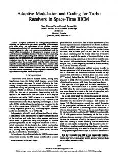
Fig. 10. 16 − QAM Performance
A. The Performance of QPSK
C. The Performance of 64-QAM
Figure 9 depicts the Bite Error Rate (BER) in term of SNR with the scenarios of QPSK modulation without and with code rates of CR = 13 , CR = 12 , CR = 23 . It is shown that the best performance occurs for CR = 31 , and the performance decreases with the increase of CR. The figure shows that for a fixed value of BER = 10−4 , the gain in SNR with coding, comparing to the modulation without coding, is equal to 5dB, 8dB and 12dB when CR = 23 , CR = 21 , CR = 13 respectively.
Figure 11 depicts the BER in term of SNR with the scenarios of 64 − QAM modulation without and with code rates of CR = 13 , CR = 12 , CR = 23 . It is shown that the best performance occurs for CR = 31 , and the performance decreases with the increase of CR. The figure shows that for a fixed value of BER = 10−4 , the gain in SNR with coding, comparing to the modulation without coding, is equal to 5dB, 10dB and 15dB when CR = 23 , CR = 12 , CR = 31 respectively.
Fig. 9. QP SK Performance Fig. 11. 64 − QAM Performance
B. The Performance of 16-QAM Figure 10 depicts the BER in term of SNR with the scenarios of 16 − QAM modulation without and with code rates of CR = 31 , CR = 12 , CR = 23 . It is shown that the best performance occurs for CR = 31 , and the performance decreases with the increase of CR. The figure shows that for a fixed value of BER = 10−4 , the gain in SNR with coding, comparing to the modulation without coding, is equal to 5dB, 9dB and 13dB when CR = 23 , CR = 21 , CR = 13 respectively.
D. Comparison of Performances The figure 12 shows that the performance of 16 − QAM with CR = 31 is better than QP SK with CR = 32 , though the number of bits per symbol is 13 in both case. The performance of 64 − QAM with CR = 13 is better than 16 − QAM with CR = 13 , though the number of bits per symbol is 2 in both cases.
38
Fig. 12. Performances of different modulation with different code rates
Fig. 15. Throughput in term of SNR in AWGN channel
Figure 13 shows the Frame Error Rate (FER) in term of SNR for different modulations and coding.
Similar results are obtained in Figure 16 that shows the throughput in the presence of AWGN channel and Rayleigh fading.
Fig. 13. Frame Error Rate in term of SNR
Figure 14 shows the minimum thresholds of SNR that allows to choose the respective modulation and coding for F ER = 10−2 . We notice that 16 − QAM with CR = 13 replaces QPSK with CR = 23 , and 64 − QAM with CR = 13 replaces 16 − QAM with CR = 12 . bpsym 2/3 1 4/3 2 8/3 3 4
SN R(dB) CR − 1/3 3 1/2 4 1/3 9 1/3 12.5 2/3 14.5 1/2 18.5 2/3
M odulation QP SK QP SK 16 − QAM 64 − QAM 16 − QAM 64 − QAM 64 − QAM
Fig. 16. Throughput in term of SNR in AWGN channel with Rayleigh fading
IV. S IMULATION OF THE A DAPTIVE M ODULATION AND C ODING
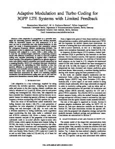
Our simulation of the adaptive modulation and coding is shown in Figure 17. The block diagram is similar to the Figure 1 with the additional Adaptation block. The demodulator at the receiver part calculates the SNR and sends it to the Adaptation block which decides the suitable modulation and coding. Figure 18 shows the curves of the throughput in term of SNR for the adaptive modulation and coding with Rayleigh fading. The curve matches the curve of QP SK and CR = 13 for low values of SNR, and matches the curves of 64 − QAM and CR = 23 for high values of SNR. For the medium value of SNR we notice a gain of 4dB at SN R = 15dB. By consequence the throughput curve of the adaptive modulation and coding acts like an envelope of the maximum values of the throughput of the static modulation and coding.
Fig. 14. The Minimum threshold for modulation and coding
E. Throughput in term of SNR for AWGN and Rayleigh fading Figure 15 shows the throughput in the presence of AWGN channel. We notice that 16−QAM with CR = 13 gives higher throughput than QP SK with CR = 23 . We also notice that 64 − QAM with CR = 31 gives higher throughput than 16 − QAM with CR = 31 .
39
Fig. 19. Throughput of AMC
Figure 19 shows the measured and the simulated throughput in term of SNR for the adaptive modulation and coding. We noticed that most of the points of the measurements are located near the throughput of the adaptive modulation and coding. Some points deviate because of the difference between the real channel and the simulated channel. VI. C ONCLUSION This paper presented the simulations of the adaptive modulation and coding for mobile communication networks. We concluded that the throughput could be increased by increasing the modulation order and the coding rate with the increase of Signal-to-Noise Ratio. The AMC gives higher throughput by changing the modulation and coding in function of the Signal-to-Noise ration at the receiver with a gain of 4dB. The simulation results are validated via drive test measurements of HSPA+ mobile network.
Fig. 17. Throughput of AMC with Rayleigh channel
R EFERENCES [1] S. Salih and M. Suliman, Implementation of Adaptive Modulation and Coding Technique using, International Journal of Scientific and Engineering Research Volume 2, Issue 5, May-2011, ISSN 2229-5518. [2] S. Kottkamp, HSPA+ Technology Introduction, Application Note, Rohde and Schwarz, 2009 [3] S. Hadi and T. Tiong, Adaptive Modulation and Coding for LTE Wireless Communication, IOP Conf. Series: Materials Science and Engineering 78, 2015. [4] M. Fernandez and M. Rupp and M. Wrulich HSDPA CQI Mapping Optimization Based on Real Network Layouts, Bachelor Thesis, Institute of Communications and Radio-Frequency Engineering, 2008. [5] F. Huang T. Pratt, Evaluation of Soft Output Decoding for Turbo Codes, Master of Science, Electrical Engineering,ETD etd-71897-15815, 1997. [6] M. Tuechler and J. Hagenauer. Channel coding, lecture script, Munich University of Technology, pp. 111-162, 2003. [7] J. Proakis, Digital Communications, fourth edition, Mc-Graw Hill, 2001 [8] P. Farrell and J. Moreira, Essentials of Error-Control Coding, John Wiley and Sons Ltd, 2006. [9] K. Bogawar, S. Mungale and M. Chavan, Implementation of Turbo Encoder and Decoder, International Journal of Engineering Trends and Technology (IJETT), Volume 8 Number 2- Feb 2014. [10] B. Sklar Rayleigh Fading Channels in Mobile Digital Communication Systems, Part I: Characterization,IEEE Communications Magazine, July 1997. [11] T. Nugraha Drive Test Nemo,Technology, Business, Aug 19, 2012.
Fig. 18. Throughput of AMC
V. VALIDATION OF THE AMC S IMULATION RESULTS To validate our simulation results of the AMC, we use Nemo outdoor and Nemo Analyze tools [11] from one of the mobile operator in the country. The tools allow to measure, store and analyze the parameters of the HSPA+ network between the Node B and the user (e.g. modulation and coding, Energy chip/Noise, Channel Quality Indicator, Number Channelization Code).
40