Journal of
Mechanical Science and Technology Journal of Mechanical Science and Technology 22 (2008) 1073~1083 www.springerlink.com/content/1738-494x
Adaptive nonlinear control using input normalized neural networks Henzeh Leeghim*, In-Ho Seo and Hyochoong Bang Korea Advanced Institute of Science and Technology (KAIST), Daejon, Korea (Manuscript Received August 8, 2006; Revised August 13, 2007; Accepted November 8, 2007) --------------------------------------------------------------------------------------------------------------------------------------------------------------------------------------------------------------------------------------------------------
Abstract An adaptive feedback linearization technique combined with the neural network is addressed to control uncertain nonlinear systems. The neural network-based adaptive control theory has been widely studied. However, the stability analysis of the closed-loop system with the neural network is rather complicated and difficult to understand, and sometimes unnecessary assumptions are involved. As a result, unnecessary assumptions for stability analysis are avoided by using the neural network with input normalization technique. The ultimate boundedness of the tracking error is simply proved by the Lyapunov stability theory. A new simple update law as an adaptive nonlinear control is derived by the simplification of the input normalized neural network assuming the variation of the uncertain term is sufficiently small. Keywords: Adaptive nonlinear control; Feedback; Linearization; Neural networks; Uncertain systems; Input normalization --------------------------------------------------------------------------------------------------------------------------------------------------------------------------------------------------------------------------------------------------------
1. Introduction As an enabling nonlinear control theory, the feedback linearization technique has been applied to a wide variety of systems. This method is called model inversion due to the basic idea of nonlinearity cancellation in the inverse model of the system. The controller is limited to the full knowledge of the nonlinear system model, and applicable only when the system is feedback linearizable. If the exact model is not known or only uncertain system information is available, the boundedness of the error and the stability of the closed loop system are not guaranteed. In this paper, the feedback linearization technique combined with an adaptive control term is proposed for the uncertain systems. One potential approach to handle the model error uncertainty, high nonlinearity, or actuator uncertainty is adaptive control. Adaptive control parameterizes the uncertainty in terms of certain unknown parameters and tries to take advantage of the feedback strategy to learn these parameters during the operation of *
Corresponding author. Tel.: +82 42 869 3758, Fax.: +82 42 869 5762 E-mail address:
[email protected] DOI 10.1007/s12206-007-1119-1
the system. If a system possesses many unknown parameters to be estimated, the adaptive control for real-time applications may not be feasible because of the computational burden involved. However, generic adaptive controls are now becoming enabling technologies due to the rapid progress in microprocessor performance. Successful advance in adaptive control has been achieved during the last several decades in various applications such as robotics, aircraft control, and estimation problems. Since the neural network was demonstrated as a universal smooth function approximator [1], extensive study has been conducted for different applications, especially pattern recognition, identification, estimation, and control of dynamic systems. [2-6] One of the crucial properties of the neural network is the weights to be optimized with certain bounded values through appropriate learning rules. Most adaptive control methods have been restricted to the systems linear in the unknown parameters, and experienced limitation from the difficulty of parameter formulations. However, learning-based controls with neural network are regarded as alternatives to adaptive control. Uncertain nonlinear terms of the systems can be modeled in terms of the neural network. In this
1074
H. Leeghim et al. / Journal of Mechanical Science and Technology 22 (2008) 1073~1083
case, the weights of the neural network are treated as the additional unknown parameters to be estimated. Lewis et al. applied adaptive control using neural network for a general serial-link rigid robot arm. [6] The structure of the neural network controller is derived by the filtered error approach. Moreover, Lewis took neural network for adaptive observer design, [7] and developed a neural network controller for the robust backstepping control of robotic systems in both continuous and discrete-time domains. [8] Calise et al. have worked extensively on the control and estimation of aircraft and helicopters using neural network. [9-13] Adaptive output feedback control using a high-gain observer and radial basis function neural network was proposed for nonlinear systems represented by input-output models. [14, 15] Also, a nonlinear adaptive flight control system was designed by backstepping and neural network controller. [16] In the previous works, stability analysis of the closed-loop system using the neural network is rather involved in mathematical development. Also, many assumptions and conditions are usually required to prove the ultimate boundedness of the tracking error. As one of the assumptions, the boundedness of reference signals is mandatory to prove the stability. The large reference signals tend to cause large boundedness of the tracking error because the assumption is closely connected to the boundedness of the tracking error. In this paper, the boundedness assumption is relaxed by using the input normalized neural network. The neural network is configured by replacing the input vector with a normalized input vector. The importance of the input data normalization is emphasized because of various benefits for function approximation. [17] The high order terms of the activation functions-sigmoidal, RBF, tanh functions - based on the input normalized neural network can be shown to be simply bounded. It is a result different from that of the previous studies. Consequently, this property leads to a simple condition for the tracking error to be ultimately bounded without the information on the trajectory bound. Furthermore, a new adaptive law is derived by the simplification of the neural network and approximation of the normalized input vector to zero on the condition that the variation of the uncertain terms is sufficiently small. The new adaptive control law provides a possibility that the uncertain error could be eliminated within a small error bound. This paper is organized into several sections. First, the background of the study of feedback linearization
and problem formulation is presented. Then, a review of the neural network and definition of the input normalization are presented with the neural network applied to the adaptive control law design for uncertain systems. In the next section, the stability analysis and a new adaptive control theorem are presented. Finally, the proposed control law is applied to an example system for demonstration purpose.
2. Background 2.1 Feedback linearization Consider a single-input-single-output nonlinear system x = F ( x ) + G ( x )u y = H ( x)
(1)
where F , G and H are sufficiently smooth functions in a domain D ⊂ R N and u , y ∈ R are the system input and output, respectively. Different nonlinear control techniques for the problem formulated in Eq. (1) have been pursued over the well-known F , G . However, it is not easy to acquire exact knowledge on F , G for complex plants. For practical problems, f , g are the best estimates for the uncertain F , G , respectively. Thus, the system is reconfigured as x = f ( x ) + g ( x )u y = h( x)
(2)
In this paper, the feedback linearization approach is applied to control the system. The derivative y of the system in Eq. (2) can be expressed in the form y=
∂h [ f ( x) + g ( x )u ] = L f h( x) + Lg h( x)u ∂x
(3)
where L f h( x) =
∂h ∂h f ( x), Lg h( x) = g ( x) ∂x ∂x
(4)
represents Lie derivatives of h with respect to f , g . (ρ ) with If the input-output relationship appears in y a nonzero coefficient such as y ( ρ ) = L(fρ ) h( x) + Lg L(fρ −1) h( x )u
(5)
Then ρ is defined as a relative degree of the system. A feedback linearized system can be transformed by change of variables as follows: η = f 0 (η , ξ )
(6)
ξ = Acξ + Bcγ ( x)[u − α ( x)]
(7)
H. Leeghim et al. / Journal of Mechanical Science and Technology 22 (2008) 1073~1083
y = Ccξ
(8)
where ξ = [ y , y ,… , y ( ρ −1) ] ∈ R ρ ,η ∈ R N − ρ , γ ( x ) = Lg L
( ρ −1) f
h( x) and α ( x) = −
L(fρ ) h( x) Lg L(fρ ) h( x)
Eq. (6) describes internal dynamics and ( Ac , Bc , Cc ) is in a canonical form.
⎡0 1 ⎢0 0 Ac = ⎢ ⎢ ⎢ ⎣0 0
0⎤ ⎡0 ⎤ ⎡1 ⎤ ⎥ ⎢ ⎥ ⎢ ⎥ ⎥ , B = ⎢ ⎥ , C = ⎢0⎥ c c ⎢0 ⎥ ⎢ ⎥ 1⎥ ⎥ ⎢ ⎥ ⎢ ⎥ 0⎦ 1 ⎣ ⎦ ⎣0 ⎦
T
(10)
Without loss of generality, we assume that f 0 (0,0) = 0 . To design a state feedback control law, a reference signal should be defined so that the output y asymptotically tracks the reference signal r (t ) . It is also assumed that the reference signal ( (r , r , …, r ( ρ ) ) ) is available on-line. For convenience, let us define two vectors as y−r ⎡ r ⎤ ⎡ ⎤ ⎢ ⎥ ⎢ ⎥ =ξ − R R=⎢ ⎥,E = ⎢ ⎥ ( ρ −1) ( ρ −1) − r ( ρ −1) ⎦⎥ ⎣⎢ r ⎦⎥ ⎣⎢ y
(11)
where R is the reference signal vector and E corresponds to an error vector. The error dynamics is derived through the change of variables from Eq. (7) such that E = Ac E + Bc {γ ( x)[u − α ( x)] − r ( ρ ) }
(12)
The nonlinear feedback control law is developed in the form u = α ( x ) + β ( x)[v + r ( ρ ) ]
Additional control action is redefined to control the uncertain terms such that u = α ( x) + β ( x)[v + r ( ρ ) − vad ]
(9)
(13)
where β ( x) = 1/ γ ( x) and v is a pseudo control input. 2.2 Problem formulation The tracking control law derived so far is based on the system dynamics in Eq. (2). However, the system to be controlled ultimately is a nonlinear system in Eq. (1). The difference between Eq. (1) and Eq. (2) induced from the model uncertainty amounts to ∆ (⋅) through feedback linearization. In other words, the reference model tracking error dynamics based on the system in Eq. (1) becomes E = Ac E + Bc {γ ( x)[u − α ( x)] − r ( ρ ) + ∆( x, u ( x))} (14)
1075
(15)
where vad represents an adaptive control term. Assumption 1 : The error dynamics in Eq. (14) is a well defined system with a relative degree ρ . The internal dynamics in Eq. (6) is Lipschitz with respect to ξ and globally exponentially stable so that there exists a Lyapunov function Vη (η ) in some neighborhood of η = 0 given by [18] c1 η ∂Vη ∂η
2 2
≤ Vη (η ) ≤ c2 η
f 0 (η ,0) ≤ −c2 η
2 2 2 2
(16) (17)
and ∂Vη ∂η
≤ c4 η
2 2
(18)
2
where c1 , c2 , c3 and c4 are positive constants. The primary goal of this study is to construct an adaptive control law to compensate the model uncertainty so that the output tracks a reference trajectory with bounded error. The baseline control law is constructed by the feedback linearization of the system in Eq. (2). A neural network is incorporated into the baseline control law to compensate for the uncertain terms. 2.3 Input normalized neural networks (INNN) Since the neural network was demonstrated as a universal smooth function approximator, there has been a wide range of applications, especially pattern recognition, identification, estimation and control of dynamic systems. Recent advance in the neural network has allowed a series of new technologies. There are several types of architecture for the neural network to solve different problems. One promising type involves input normalized neural networks (INNN) which are configured by replacing the input vector of the neural network with a normalized input vector. An adequate normalization of the input vector is a linear scale conversion that assigns the same absolute value to the corresponding relative variation. The effect of input data pre-treatment prior to the neural network training is demonstrated by systematic analy-
1076
H. Leeghim et al. / Journal of Mechanical Science and Technology 22 (2008) 1073~1083
1
1
⎡ bv1 ⎢v V = ⎢ 11 ⎢ ⎢ ⎣vn1
y
x V
σ (υ ) = [1 ϑ (υ1 )
Fig. 1. A three-layered neural network architecture.
sis. The importance of the input data normalization is emphasized due to several advantages for function approximation. [17] One advantage is that the estimation error can be reduced. Another merit lies in the calculation time reduced in the order of magnitude for the training process. This approach provides also an improved capability in discriminating high-risk software. [19] From control theory viewpoint, the INNN provides several advantages as well as the advantage of the neural network itself as it will be discussed later. A general three-layered neural network architecture illustrated in Fig.1 consists of a large number of parallel interconnections of neural processors. The threelayered neural network consists of an output vector ( y ∈ R l ) about the input vector ( x ∈ R n ) as follows:
(20)
where σ denotes an activation function vector. The bias terms bvi , bwi are absorbed into V and W , respectively, by redefining the input vector of the neural network.
χ = [1 x ]
T
(22)
ϑ (υm )]
T
(23)
where υi denotes the i-th element of the vector V T χ ∈ Rm . The INNN can be easily implemented by defining the normalized input vector as follows: z=s
χ χ
(24)
where s is a positive scaling parameter. Thus, the 2norm of the normalized input vector simply satisfies z =s
(25)
Remark. 1 The ideal weight matrices of the neural network are unknown and possibly non-unique, which implies that the weights can be optimized to satisfy desired design objectives. This is possible by judicious selection of each learning rate of the weights and initial values.
(19)
where wij ∈ R is the interconnection weight between the hidden and output layers, ϑ denotes an activation function. In addition, v jk ∈ R is the interconnection weight between the input and hidden layers while bvi and bwi are bias terms. The neural network in this architecture is generally known as the universal approximator for continuous nonlinear functions. The output function can be expressed in a simpler form as y = W T σ (V T x)
bwl ⎤ w1l ⎥⎥ ⎥ ⎥ wml ⎦
where V ∈ R ( n +1)× m ,W ∈ R ( m +1)×l . The activation function vector is described as
W
m ⎡ ⎤ ⎛ n ⎞ yi = ∑ ⎢ wijϑ ⎜ ∑ vik xk + bvj ⎟ + bwi ⎥ j =1 ⎣ ⎝ k =1 ⎠ ⎦
bvm ⎤ ⎡ bw1 ⎢w v1m ⎥⎥ ,W = ⎢ 11 ⎥ ⎢ ⎥ ⎢ vnm ⎦ ⎣ wm1
(21)
For the simple form of the neural network, the elements of the two weight matrices are defined as
Remark. 2 An input normalized neural network possesses some useful advantages such that the estimation error, the computational time for the training process, and other risks can be reduced. Assumption 2. There are ultimately converged ideal weights (constant matrices) at the end of the learning process and the following bounds hold V ≤V, W ≤W
(26)
where V ,W are the upper bounds of the unknown weight norms. A suitable choice of neurons is needed to represent a nonlinear function with converged constant weights. That is, careful consideration for the significance of the nonlinearity is required to satisfy both the approximation property and assumption 2.
H. Leeghim et al. / Journal of Mechanical Science and Technology 22 (2008) 1073~1083
3. Adaptive controller design
the activation vector such that
The reference model tracking error dynamics in Eq. (14) is expressed as E = Ac E + Bc {γ ( x)[u − α ( x)] − r ( ρ ) + ∆( x, u ( x))} (27)
and the pseudo control input is defined as vad = − KE , where K T ∈ R ρ is a feedback gain matrix. Inserting the control input in Eq. (15) into Eq. (27), the error dynamics are modified into E = Ac E + Bc {−vad + ∆ ( x, u ( x))}
(28)
where A = Ac − Bc K and the gain matrix is selected so that A becomes Hurwitz. For this, there exists a positive definite matrix satisfying AT P +PA = −Q
(29)
The Lyapunov equation guarantees a unique positive definite solution. The INNN is applied to compensate for the model uncertainty so that the model uncertainty of the system can be replaced by ∆ ( x, u ( x)) = W T σ (V T z ) + ε
(30)
where ε represents a function reconstruction error. In general, given a constant real number ε > 0, ∆ ( x, u ( x)) is within ε range of the neural network. It was remarked in the previous section that the neural network has constant weight matrices at the end of the learning process. From this statement, the representation in Eq. (30) holds with ε < ε . The adaptive control term is required to satisfy vad = Wˆ T σ (Vˆ T z )
(31)
where Wˆ ,Vˆ are on-line estimates of W ,V 9 , respectively, such that V = V − Vˆ W = W − Wˆ
(32)
The estimated weights are updated by the update rules: Vˆ = LzWˆ Tσ ′(Vˆ T z)( ET PBc ) − kLVˆ Wˆ = M ( ET PBc ) ⎣⎡σ (Vˆ T z ) − σ ′(Vˆ T z)Vˆ T z ⎦⎤ − kLWˆ
1077
(33)
Note that k is a design parameter, ( L, M ) are positive definite learning rate matrices, and σ ′(υ ) denotes a Jacobian matrix containing derivatives of
⎡ 0 ⎢ ∂ϑ (υ ) 1 ⎢ ⎢ ∂v1 σ ′(υ ) = ⎢ ⎢ ⎢ ⎢ 0 ⎣⎢
⎤ ⎥ 0 ⎥ ⎥ m ⎥ ,υ ∈ R ⎥ ∂ϑ (υ m ) ⎥ ⎥ ∂vm ⎦⎥ 0
(34)
The Taylor series expansion of σ (V T z ) for a given T
V z
yields
σ (V T z ) = σ (Vˆ T z ) + σ ′(Vˆ T z )V T z + O(V T z ) 2 T
(35)
2
where O(V z ) denotes terms of order two. Lemma.1 For sigmoid, RBF, and tanh functions as the activation functions of the INNN, the higher order terms in the Taylor series are bounded by O(V T z ) 2 ≤ c5 + c6 s V
(36)
where c5 , c6 are positive constants. PROOF : From Eq. (35) and some norm inequality in conjunction with the fact that the activation function and associated derivatives are bounded by constants, the higher order terms are also bounded such that σ (V T z ) = ⎡⎣σ (V T z ) − σ (Vˆ T z ) ⎤⎦ − σ ′(Vˆ T z )V T z (37) ≤ c5 + c6 V z Finally, Lemma.1 is derived by substituting the INNN property in Eq. (25) into Eq. (37). The following inequality provides useful properties for the stability analysis W T σ ′(Vˆ T z )V T z ≤ d1s W (38) W T O(V T z ) 2 ≤ d 2 + d3 V where d1 , d 2 and d 3 are computable positive constants. The inequalities are readily derived from Lemma.1 and Eq. (26). For the stability analysis, Eq. (35) is substituted into Eq. (30). Consequently, the difference between the on-line output of the neural network and the model uncertainty satisfies the following relationship: −vad + ∆( x, u ( x)) = −Wˆ Tσ (Vˆ T z ) + W Tσ (V T z ) + ε = W T ⎡⎣σ (Vˆ T z ) − σ ′(Vˆ T z )Vˆ T z ⎤⎦ +Wˆ Tσ ′(Vˆ T z )V T z + δ
(39)
1078
H. Leeghim et al. / Journal of Mechanical Science and Technology 22 (2008) 1073~1083
(
where
+tr −WT ET PBc ⎡⎣σ (VˆT z) − σ ′(VˆT z)Vˆ T z⎤⎦ + kWTWˆ
δ = W T σ ′(Vˆ T z )V T z + W T O(V T z ) 2 + ε From Eq. (38), one can show that δ is also bounded by
δ ≤ d 4 + d1s W + d3 s V
(40)
where d 4 = d 2 + ε is additional positive constant.
(
+tr −V zWˆ σ ′(Vˆ z)E PBc + kV Vˆ T
T
T
T
)
Stability of the error dynamics combined with the INNN is discussed in this section. The stability analysis is based on the Lyapunov direct method. The full states including the weights of the INNN should be used because of the on-line function approximation rules. Theorem. 1 First, let the assumptions 1 and 2 hold. Then, the control input of the error dynamics satisfies u = α ( x) + β ( x)[v + r ( ρ ) − Wˆ Tσ (Vˆ T z )]
(41)
λmin (Q)k > a02 s 2
xT y = tr ( xT y ) = tr ( xyT )
(46)
VL = − E T QE + E T PBcδ + tr (kW TWˆ + kV TVˆ )
PROOF: Let us examine the following candidate Lyapunov function for the system in Eq. (27) 1 1 1 VL = E T PE + tr W T M −1W + tr V T L−1V 2 2 2
(
)
VL
(
)
(43)
by inserting Eq. (27)
VL = ET ( AT P + PA) E + ET PBc (−vad + ∆( x, u ( x)) +tr (W T M −1W ) + tr (V T L−1V )
2
VL ≤ −λmin (Q) E + ET PBc (d4 + d1s W + d3s V ) +tr (kW TWˆ + kV TVˆ )
VL ≤ −λmin (Q) E
2
+ λmax ( P)(d1s W + d3 s V ) E −k ( W
2
(49)
2
+ V )
+ λmax ( P) d 4 E + kW W + kV V
For convenience, some notations are introduced as 2a0 = max ⎡⎣ λmax ( P )d1 a1 = max ⎡⎣ λmax ( P) d 4
λmax ( P) d3 ⎤⎦ kW
(50)
kV ⎤⎦
and Z = ⎡⎣ V
W ⎤⎦
T
(51)
where a1 is a positive constant. From the norm property such that β
≤ cn 2 x α
(52)
Eq. (49) results in 2
Here the difference between the on-line output of the neural network and model uncertainty is replaced with Eq. (39). Then by making use of the neural network update rules in Eq. (33), the time derivative of VL becomes
(48)
can be derived. Applying the upper bounds of the weight matrices from Eq (26), the time derivative of VL can be rewritten as
cn1 x α ≤ x
(44)
(47)
If we use Eqs. (32) and (40), then
(42)
where a0 is a positive constant. The tracking error and the weight error of the INNN are ultimately bounded.
{
(45)
Since A is Hurwitz, there exists a symmetric positive definite solution, and from the trace equality property such as
The update rules of the INNN are described in Eq. (33), and a condition satisfies the following inequality:
VL = ET ( AT P + PA)E
)
one can obtain the time derivative of VL written as
4. Stability analysis
The time derivative of produces
T
VL ≤ −λmin (Q ) E + 2a0 s E Z − k Z
2
+ a1 ( Z + E ) T
⎡ E ⎤ ⎡λ (Q ) − a0 s ⎤ ⎡ E ⎤ = − ⎢ ⎥ ⎢ min ⎢ ⎥ k ⎦⎥ ⎢ Z ⎥ ⎢⎣ Z ⎥⎦ ⎣ − a0 s ⎣ ⎦
(53)
+ a1 ( Z + E )
}
+ET PBc ⎡WT σ (VˆT z) − σ ′(VˆT z)Vˆ T z + Wˆ Tσ ′(VˆT z)V T z + δ ⎤ ⎣ ⎦
Once again, we redefine a matrix and a vector as
H. Leeghim et al. / Journal of Mechanical Science and Technology 22 (2008) 1073~1083
edness can be also small by choosing small s.
⎡E⎤ ⎡λ (Q ) − a0 s ⎤ ,L = ⎢ ⎥ QL = ⎢ min ⎥ k ⎦ ⎢⎣ Z ⎥⎦ ⎣ − a0 s
where the matrix ( QL ) can be a symmetric positive definite matrix and satisfies the condition in Eq. (42) by a proper selection of k , s and Q . Consequently, Eq. (53) is simplified into 2
VL ≤ −λmin (Q ) L + a1 L
(54)
and the following condition ∀ L >
a1 λmin (QL )
(55)
renders VL < 0 outside a compact set. According to the Lyapunov stability theory, this result verifies the uniform ultimate boundedness of L . Remark 3 The control theories based upon neural network studied in the past generally required boundedness of the desired trajectory. [5, 9, 13, 16] The assumption is also directly related to the tracking error boundedness so that larger boundedness of the desired trajectory produces larger tracking and weight errors. In practical applications, the trajectory and its derivatives up to r ( ρ ) (t ) should be bounded for all t ≥ 0 . However, this assumption may be unnecessary for controller design and stability analysis. In this study, the seemingly unnecessary assumption is avoided by employing the INNN technique. Remark 4 The ultimate boundedness is derived from the candidate Lyapunov function in Eq. (43). The condition in Eq. (42) is also necessary to make a positive definite matrix in the stability analysis. The Lyapunov stability theory satisfies only the sufficient condition so that there may exist several conditions to create ultimate boundedness satisfying VL < 0 with different Lyapunov functions. In this paper, it can only be concluded that the condition in Eq. (42) leads to the ultimate boundedness based on the Lyapunov function in Eq. (43). Remark 5 The ultimate boundedness of the tracking and weight errors can be made smaller by properly controlling the parameters. The larger the Q , the smaller boundedness tends to result. Occasionally, the bound-
1079
k and
Remark 6 The selection of the feasible parameters is very important. Basically, k , M and L should be specified based on the neural network property so that assumption 2 holds. The sufficiently large Q is recommendable considering the degree of uncertainty, and then the parameter s is selected satisfying the constraint in Eq. (42). Theorem. 2 Let assumption 1 and Eq. (42) hold true. It is also assumed that the variation of the modeling uncertainty ∆ ( x, u ( x)) is small enough. The adaptive control input of the error dynamics can be approximated such as u = α ( x) + β ( x)[v + r ρ − φˆ]
(56)
where φˆ denotes the best estimate of the scalar neural network. The corresponding update rule is given by
φˆ = kE T PBc − kφˆ
(57)
where k is a scalar learning rate. Then, the tracking error and the scalar neural network error are ultimately bounded. PROOF : Stability analysis is basically equivalent to that of Theorem 1. By controlling s , the update rules in Eq. (33) can be approximated into a simple form. That is, the input of the activation function approaches zero from Eq. (25) as s → 0 . The activation function and its derivative will also be approximately constants. As the ideal weight matrices are generally unknown and possibly non-unique, the neural network may reach another ultimately converged ideal weight such as V ≤ V1 , W ≤ W1
(58)
where V1 ,W1 represent another possibly maximum positive constants. Applying the activation function being close to a constant and the zero input, a new update rule is obtained by Wˆ ≈ ME T PBcσ (0) − kMWˆ
(59)
Updating Vˆ is not necessary as it can be seen from Eq (33) with the approximation of s ≈ 0 . Because the weights with the same initial values and gains can be approximated to a weighted scalar pa-
1080
H. Leeghim et al. / Journal of Mechanical Science and Technology 22 (2008) 1073~1083
rameter and the assumption of the small variation, the adaptive input can be approximated as vad ≈ Wˆ T σ (0) = φˆ
(60)
y1 = y2 y2 = −ωn2 y1 − 2ζωn y2 + ωn2 µ (t ) r = y1
The results in Eqs. (59)-(60) verify theorem 2. The approximated control law is derived from theorem 1 for the adaptive control under high-level uncertain nonlinearity. Theorem 2 provides a possibility for the uncertain nonlinear error to be eliminated by using the scalar neural network analogous to the general integral control.
Therefore, if µ (t ) is a piecewise continuous function of time, r (t ), r (t ) and r (t ) are available on-line. Fig. 2 shows the reference signal trajectory with ωn = 2 and ζ = 0.9 , respectively. From the following definition
5. Simulation study
the tracking error dynamics satisfy
To demonstrate the nonlinear control approach for uncertain nonlinear systems, a simple pendulum equation is considered here. x1 = x2
⎡x − r⎤ E=⎢ 1 ⎥ ⎣ x2 − r ⎦
e1 = e2 e2 = − a sin x1 + bx2 + cu − r y = x1
The state feedback control from Eq. (13) yields
x2 = − a sin x1 + bx2 + cu
u=
y = x1
where a, b and c are constants. The system has a relative degree of two in R 2 and represented in the normal form. It has no nontrivial zero dynamics so that the pendulum system has basically minimum phase characteristics and satisfies assumption 1. A reference signal r(t) and its derivative should be specified. For the system with a relative degree of two, the transfer function of the reference model is modeled as a second-order linear time-invariant system represented by
ωn2 s 2 + 2ζωn s + ωn2 where the positive damping ratio ζ and the natural frequency ω are judiciously chosen to shape the reference signal r (t ) for a given command µ (t ) . The reference signal can be also generated on-line from the state model:
1 [ a sin x1 − bx2 + r − k1e1 − k2e2 ] c
where K = [k1 , k2 ]T is designed to assign the eigenvalues of Ac − Bc K at the desired location in the left-half complex plane. However, if the system is unknown, thus at most the estimated system only is available, then the best estimated system function may replace the original system in the state feedback control law. Eq. (41) such that u=
1 ⎡ a sin x1 − bx2 + r − k1e1 − k2e2 − vad ⎤⎦ c⎣
where a , b and c are the best estimates of a, b and c , respectively. For the simulation, a = b = 10 and c = 1 are assumed for the nominal system while a = 7, b = 1.4 and c = 6 for the best estimated system. Feedback gains are set to be k1 = 5 and k2 = 1 . The architecture of the neural network consists of five hidden neurons and the following sigmoid function as the activation function is adopted:
6
r r' r''
4
ϑ ( z) =
1 1 + e− z
Reference inputs
2
Learning rate matrices were set to L = 0.1I , M = I and k = 0.1 , respectively. To satisfy the con-
0 -2 -4 -6
0
10
20
30
time (sec)
Fig. 2. Reference input histories.
40
50
dition in Eq. (42), the input scaling parameter is set to s = 0.5 with enough margin. The initial INNN weights are set to zeros. Fig. 3 shows the tracking performance and control history without the INNN strategy. The solid curve is
1081
H. Leeghim et al. / Journal of Mechanical Science and Technology 22 (2008) 1073~1083 3
6
2
4
1
2
W weights
Tracking
0 -1 -2
exact case uncertain case
-3 -4
0
10
ki
hi
b
20
30
40
-6
50
l k
d
i
0
10
20
30
40
50
time (sec)
dd d
(a) Tracking history between exactly known case and uncertainty added case
(a) Interconnecton weight between hidden and output layers 3.0x10⁻³
3
2.0x10⁻³
2
1.0x10⁻³
V weights
1
control inputs
-2 -4
time (sec)
)T
0
0
0.0
-1.0x10⁻³
-1
-2.0x10⁻³ -2
-3.0x10⁻³ -3
0
10
20
30
40
50
time (sec)
0
10
20
time (sec)
30
40
50
(b) Interconnection weight between input and hidden layers
(b) Control input history corresponding to the control laws
Fig. 5. INNN weights update history.
Fig. 3. Tracking performance without INNN augmentation. 3 2
Tracking
1 0 -1 -2
Reference signal With INNN
-3 -4
0
10
20
30
40
50
time (sec)
(a) Tracking history between exactly known case and uncertainly added case 3 2
control input
1 0 -1 -2 -3 0
10
20
30
40
50
time (sec)
(b) Control input history corresponding to the control laws Fig. 4. Tracking performance with INNN augmentation.
the output of the system in the nominal case. As one can see, the tracking is achieved for all t ≥ 0 asymptotically. The dotted curve also denotes the output signal when the model parameter is perturbed and the modeling error is added. Oscillation is introduced due to the model uncertainty. Fig. 4 presents the simulation results achieved with the INNN augmented. The system tracks the reference inputs with a small error bound without oscillation. The oscillation induced to the uncertain terms is eliminated. The response by the INNN could be demonstrated in the control history. Fig. 5 presents the time history of the INNN weights. As one can see, V is very small, and this implies that the small values of V derived from Eq. (55) could make the small boundedness of the tracking error. The performance of the on-line scalar neural network is shown in Fig. 6. The scalar neural network can also control the uncertain system with a small bounded tracking error. Finally, the first result in Fig.7 shows a relationship between the number of neurons and the system with high uncertainty. The solid curve represents the output for the case of a large number of neurons (30 neurons). On the contrary, the dotted curve denotes the output for the case of a small number of neurons
1082
H. Leeghim et al. / Journal of Mechanical Science and Technology 22 (2008) 1073~1083 3
rons are required for highly uncertain systems in order to satisfy assumption 2. The solid curve in the second figure shows a case: the condition in Eq. (42) is satisfied with s = 0.5 . The diverging dotted curve at 30 sec shows a case of the violation with s = 50 .
2
Tracking
1 0 -1 -2
Reference signal With SNN
-3 -4
0
10
6. Conclusion
20
30
40
50
time (sec)
(a) Tracking history under an uncertainly added case 1.5 1.0 0.5
phi
0.0 -0.5 -1.0 -1.5 -2.0 0
10
20
30
40
50
time (sec)
(b) Sclar weight history corresponding to the control law Fig. 6. Tracking performance with scalar neural network augmentation.
In this paper, a new adaptive control approach for uncertain systems is proposed using input normalized neural network technique. The input bound assumption, which is widely used in many studies but may be unnecessary, is avoided in this study by relying on the input normalized neural network. With a simple condition, the ultimate boundedness of the tracking error regardless of the reference signals is verified through the Lyapunov stability theory. A new scalar update law is derived by simplifying the neural network under the assumption that the uncertain system is subject to sufficiently small error variation. It naturally leads to a possibility that the small uncertain error could be eliminated by the scalar neural network. Finally, the proposed control law performance was successfully validated through nonlinear simulations
8 6
Acknowledgments
4
The present study was supported by National Research Lab. (NRL) Program (2002, M1-0203-000006) by the Ministry of Science and Technology, Korea. The authors fully appreciate the financial support.
Tracking
2 0 -2 -4 -6 -8
0
10
20
30
40
50
time (sec)
References
(a) Comparison in accordance with number of neurons 3 2
Tracking
1 0 -1 -2 -3 0
10
20
30
40
50
time (sec)
(b) Comparison between scale parameter variations Fig. 7. System performance in accordance with parameter variation.
(10 neurons). From the simulation results, one can easily understand that an appropriate number of neu-
[1] K. Hornik, M. Stinchcombe and H. White, Multilayer feedforward networks are universal approximators, Neural Networks, 2 (5) (1989) 359-366. [2] W. L. Slotine, Neural network control of unknown nonlinear controller, Proceedings of American Control Conference, Pittsburgh, PA, (1989), 1136-1141. [3] F. L. Lewis, S. Jagannathan and A. Yesildirek, Neural Network Control of Robot Manipulators and Nonlinear Systems, Taylor & Francis Inc, (1999) 277-285. [4] F. C. Chen and C. C. Liu, Adaptively controlling nonlinear continuous time systems using multilayer neural networks, IEEE Transactions on Automatic Control, 39 (6) (1994) 1306-1310. [5] A. Yesildirek and F. L. Lewis, Adaptive feedback linearization using efficient neural networks, Jour-
H. Leeghim et al. / Journal of Mechanical Science and Technology 22 (2008) 1073~1083
nal of Intelligent and Robotic Systems, 31 (2001) 253-281. [6] F. L. Lewis, A. Yesildirek and K. Liu, Multilayer neural-net robot controller with guaranteed tracking performance, IEEE Transactions on Neural Networks, 7 (2) (1996) 388-399. [7] F. L. Lewis, K. Liu and A. Yesildirek, Control of Robot Manipulators, Macmillan, New York (1993). [8] S. Jagannathan and F. L. Lewis, Robust backstepping control of robotic systems using neural networks, Journal of Intelligent and Robotic Systems, 23 (1998) 105-128. [9] A. J. Calise, N. Hovakimyan and M. Idan, Adaptive output feedback control of nonlinear systems using neural networks, Automatica, 37 (8) (2001) 12011211. [10] A. J. Calise, Neural networks in nonlinear aircraft flight control, IEEE Aerospace and Electronic Systems Magazine, 12 (7) (1996) 5-10. [11] A. J. Calise, S. Lee and M. Sharma, Development of a reconfigurable flight control law for a tailless aircraft, Journal of Guidance, Control, and Dynamics, 24 (5) (2001) 869-902. [12] A. J. Calise and R. T. Rysdyk, Nonlinear adaptive flight control using neural network, IEEE Control System Magazine, 18 (6) (1998) 14-25.
1083
[13] N. Hovakimyan, F. Nardi and A. J. Calise, Adaptive output feedback control of uncertain nonlinear systems using single-hidden-layer neural networks, IEEE Transactions on Neural Networks, 13 (6) (2002) 1420-1431. [14] H. K. Khalil, Adaptive output feedback control of nonlinear systems represented by input-output feedback, IEEE Transactions on Automatic Control, 41 (2) (1996) 177-188. [15] S. Seshagiri and H. K. Khalil, Output feedback control of nonlinear systems using rbf neural networks, IEEE Transactions on Neural Networks, 11 (1) (2000) 69-79. [16] T. Lee and Y. Kim, Nonlinear adaptive flight control using backstepping and neural networks controller, Journal of Guidance, Control, and Dynamics, 24 (4) (2001) 675-682. [17] J. Sola and J. Sevilla, Importance of data normalization for the application of neural networks to complex industrial problems, IEEE Transactions on Nuclear Science, 44 (3) (1997) 1464-1468. [18] H. K. Khalil, Nonlinear Systems, 3rd Ed., PrenticeHall, New Jersey, (1996). [19] D. E. Neumann, An enhanced neural network technique for software risk analysis, IEEE Transactions on Software Engineering, 28 (9) (2002) 904-912.