IEEE TRANSACTIONS ON CIRCUITS AND SYSTEMS—I: FUNDAMENTAL THEORY AND APPLICATIONS, VOL. 47, NO. 4, APRIL 2000
545
Adaptive Weighted Least Squares Algorithm for Volterra Signal Modeling Steven C. K. Chan, Student Member, IEEE, Tania Stathaki, and Anthony G. Constantinides, Fellow, IEEE
Abstract—This paper presents a novel algorithm for least squares (LS) estimation of both stationary and nonstationary signals which arise from Volterra models. The algorithm concerns the recursive implementations of the method of LS which usually have a weighting factor in the cost function. This weighting factor enables nonstationary signal models to be tracked. In particular, the behavior of the weighting factor is known to influence the performance of the LS estimation. However, there are certain constraints on the weighting factor. In this paper, we have reformulated the LS estimation with the commonly used exponential weighting factor as a constrained optimization problem. Specifically, we have addressed this constrained optimization using the Lagrange programming neural networks (LPNN’s) thereby enabling the weighting factor to be adapted. The utility of our adaptive weighted least squares (AWLS) algorithm is demonstrated in the context of Volterra signal modeling in stationary and nonstationary environments. By using the Kuhn–Tucker conditions, all the LS estimated parameters may be shown to be optimal.
model [10]. In 2-D channel equalization, the Volterra model is shown to offer improved performance over linear models [11]. Other 2-D applications of the Volterra model include the edge preservation in noise smoothing of images [12], the prediction of television image sequences [13], and the contrast enhancement of noisy images [14]. The Volterra series is a generalized extension of the linear series and can be regarded as a general Taylor series of a function with memory [3]. A discrete time Volterra series with infinite memory has the expression
Index Terms—Least square estimation, neural networks, nonlinear signal modeling, Volterra system.
I. INTRODUCTION
S
IGNAL modeling based on Volterra models has been well developed and successfully utilized in many diverse applications. Several examples exist in the literature [10]. For instance, in the quadratic phase coupling phenomenon [1], [2], two harmonic components interact and produce terms in the power spectrum at their sum and difference frequencies. This is observed, for example, as the low-frequency drift oscillations of a barge, moored in a random sea [3]. Kim and Powers have demonstrated the use of an adaptive second-order Volterra filter in modeling the response of a moored tension leg platform [4]. In many instances, the Volterra model is used as a tool for the analysis and compensation of nonlinear systems. For example, the nonlinearities that are introduced into a digital transmission channel when the satellite power amplifiers are driven near their saturating point are analyzed and compensated using a Volterra model [5], [6]. The Volterra model has also shown improvement over linear models in the detection of signals obscured by noise [7]. In array processing, the detection of the signal source has been investigated using a Volterra model in [8] and [9]. There are also various two-dimensional (2-D) applications of the Volterra Manuscript received September 7, 1997; revised October 19, 1998. This paper was recommended by Associate Editor J. Goetze. The authors are with the Signal Processing and Digital Systems Section, Department of Electrical and Electronic Engineering, Imperial College of Science, Technology, and Medicine, London SW7 2BT, U.K. (e-mail:
[email protected]). Publisher Item Identifier S 1057-7122(00)02921-4.
(1) where input signal; output of the model; bias coefficients; linear coefficients; quadratic coefficients; cubic coefficients. In most signal modeling schemes, an error signal is described and the output as the difference between a desired signal . The modeling of Volterra signals, signal, involve a minimization of the error, such as in the method of least squares (LS). The modeling of signals based on the Volterra model requires excessive computational resources because the number of coefficients to be determined (1) increases exponentially with the model’s degree of nonlinearity and the Volterra filter length. Even after taking into consideration the symmetry of the second- and higher order kernels, many researchers have regarded the complexity of the Volterra model as its disadvantage [15]. Neural networks have been proposed to overcome this difficulty, especially in real-time implementations. Indeed, neural networks have been widely applied to nonlinear signal modeling because of their capability to compute in parallel, their ability to distribute a complicated processing task to the various neurons and their robustness [16]. For example, the
1057–7122/00$10.00 © 2000 IEEE
546
IEEE TRANSACTIONS ON CIRCUITS AND SYSTEMS—I: FUNDAMENTAL THEORY AND APPLICATIONS, VOL. 47, NO. 4, APRIL 2000
multilayer or feedforward neural network which represents static nonlinear maps is investigated by various researchers such as Narendra and Parthasarathy [17], Nguyen and Widrow [18], and Kuschewski et al. [19]. Recurrent neural networks have also been widely used in nonlinear signal modeling and system identification because they offer a generic representation of dynamical feedback systems [20]. The Hopfield network, which is an important member of the class of recurrent networks, is used in nonlinear signal modeling as reported by Sanchez [21] and Chu et al. [22]. In 1992, Zhang and Constantinides [23] introduced the Lagrange programming neural network (LPNN) which is based on the Lagrange multiplier method for constrained optimization. The LPNN is used for solving optimization problems with constraints without imposing any restrictions on the form of the cost function. Applications include blind Volterra system modeling [24] and in solving the satisfiability problems of propositional calculus [25]. Essentially, in nonlinear signal modeling using neural networks, the problem is twofold: the selection of the model architecture and the selection of the learning algorithm [26]. With regard to the former, it is sufficient for the purpose here, to consider the second-order Volterra model with fiin (2) nite memory
In this paper, we develop the adaptive weighted least squares (AWLS) algorithm and demonstrate its application in the modeling of both stationary and nonstationary Volterra signals. In the recursive implementations of the LS criterion, a weighting factor is commonly introduced into the objective function shown in (3) [38]. Note that the length of observable data is variable (3)
The weighting factor
has the following constraints: (4)
ensures that the data in the The weighting factor distant past are forgotten, in order to allow the possibility of tracking statistical variations in the observable data, especially when the signal to be modeled is nonstationary. One such form of weighting that is commonly used is the exponential weighting factor, defined in (5). is commonly referred to as the forgetting factor (5)
(2)
In the selection of the learning algorithm, the LS criterion [17], [18] and the least mean square (LMS) criterion [19], [26] are typically used as objective functions. Most of the work in adaptive Volterra filters, for example [27]–[29], tend to employ an LMS algorithm. However, as pointed out by Mathews and Lee [30], the slow convergence of the LMS algorithm is unacceptable in many applications. For rapid convergence, the recursive implementation of the method of LS, in particular the recursive least squares (RLS) algorithm, has been considered [31]. A direct implementation of the RLS algorithm is computationally complicated. To address this, fast RLS adaptive second-order Volterra filters have been recently presented [30], [32]. The RLS algorithm has the additional feature of being able to track slow time variations in the system parameters ( , , ), owing to the exponential weighting (windowing) technique used in its formulation. An alternative mechanism for tracking time varying system parameters is provided by a finite window length, used in algorithms known as the sliding window covariance algorithms [33]. For such nonstationary environments, these algorithms are very well researched for the linear filter [34]–[36]. However, for the case of tracking nonstationary and nonlinear systems adaptively, very little work has been done and this may be due to the high computational complexity involved [30]. Nerrand et al. [37] have studied gradient descent techniques for neural networks that undergo continual adaptation for applications in nonlinear adaptive filtering.
, for , Note that is chosen such that satisfies the constraints in (4). Note that when so that , the objective function becomes the ordinary method of least affects squares. As discussed by Haykin in [38], the use of the recursive LS estimation drastically. In addition, Cioffi and Kailath [33] have mentioned that a fixed slightly less than unity enables the slow time variations in the system parameters to be tracked. Furthermore, we shall consider the exponentially weighted least squares (EWLS) estimation as a constrained optimization and address this optimization using the Lagrange programming neural networks. II. DEVELOPMENT OF THE AWLS ALGORITHM The optimization problem is to minimize the following EWLS cost function (6)
for
subject to the following constraints: (7) (8)
Essentially, we solve this constrained optimization using the LPNN. In this case, the forgetting factor is considered as a primal variable. The treatment is to first convert the inequality
CHAN et al.: ADAPTIVE WEIGHTED LEAST SQUARES ALGORITHM FOR VOLTERRA SIGNAL MODELING
constraints into equality constraints by introducing suitable auxiliary variables and into the constraint functions, as in (9) and (10)
547
is time varying but for simplicity,
is represented by
(9) (10) The differential of the constraint functions have the following expressions: (11) (12) Next, a Lagrangian function is formulated with the introduction of Lagrange multipliers for each of the constraint func. We furtions. The dimensionality of the problem is ther convexify the Lagrangian function by introducing a penalty parameter into the Lagrangian function, as shown in (13). According to Zhang and Constantinides [23], this technique relaxes the conditions for global stability. In [23], the effects of were also studied and it was concluded that can hasten the convergence of the algorithm during the initial stages because it forces the state to approach the feasible region quickly. However, a large forces the constraint functions in the augmented term of the Lagrangian function to be very small, especially when the system state approaches the optimum solution. This may lead to finite precision errors and cause inaccuracies in the system state. In general, may be adjusted using a simple rule such , without reservation
(14) The summation of past error values makes the calculation of the gradient unnecessarily complicated. To avoid this complicaand is introduced as tion, a recursion rule involving follows:
(15)
(13)
(16) Hence
III. NEURAL ADAPTATION The forgetting factor, bias, linear, quadratic, and auxiliary variables are all primal neurons. By the definition of the LPNN, these neurons are adapted using a steepest descent rule, the gra, , dients are calculated for example , , , , , , , , , , and so forth. In contrast, the Lagrangian neurons follow a steepest ascent rule to meet the saddle point criteria. In any case, these gradient-based algorithms involve the introduction of a stepsize parameter into the update equation of the neurons.
(17) The computation of the gradient is simplified to the following form which is suitable for implementation
A. Forgetting Factor At each time instant we minimize the cost function in (13), . We use the steepest deby selecting an optimal value for scent rule for the adaptation of . It is necessary to find the gradient of Lagrangian function with respect to . This is derived is in (14). Note that for the first summation, the term at zero and so can be removed from the summation. Note also that
(18) where
,
are defined in (11) and (12).
548
IEEE TRANSACTIONS ON CIRCUITS AND SYSTEMS—I: FUNDAMENTAL THEORY AND APPLICATIONS, VOL. 47, NO. 4, APRIL 2000
By isolating the th term, the following recursion rule is found:
The forgetting factor, , is updated according to (19)
(19)
and
are updated according to (20) and (21), respec-
(28)
tively (20)
Simplifying, the gradient is updated using (29)
(21) (29) B. Volterra Kernel Neurons Using the steepest descent rule, the Volterra kernel neurons are updated by the (22)–(24)
3) Quadratic Kernel: Similarly, the derivation of the gradient of the Lagrangian function with respect to the quadratic coefficients is shown in (30)
(22) (30) (23) (24)
A recursion rule is defined by isolating the th term
, , and are deterThe gradients mined as follows. 1) Bias Term: The gradient with respect to the bias neuron is derived in (25)
(31) (25) Hence, the gradient can be updated using (32), without the need to recalculate previous values of the error Using a recursion rule, the gradient at the be updated using (26)
th instant can (32) (26) C. Auxiliary Variables
In order to elucidate the adaptation process, at time instance , and are available to calculate , by (22). which is then used to calculate 2) Linear Kernel: The linear neurons are updated similarly to the bias neuron by first determining the gradient of the Lagrangian function with respect to the linear coefficients. This is derived as follows:
The auxiliary variables are primal neurons and are updated by first finding the gradient of the Lagrangian function with respect as follows: to the auxiliary variables ,
(33)
(34) (27)
Then, the auxiliary variables may be updated using the gradient
CHAN et al.: ADAPTIVE WEIGHTED LEAST SQUARES ALGORITHM FOR VOLTERRA SIGNAL MODELING
549
TABLE I COEFFICIENTS FOR SECOND-ORDER VOLTERRA SIGNAL GENERATOR
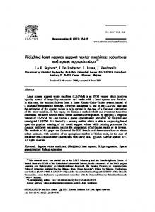
Fig. 1.
Adaptive Volterra signal modeling using LPNN.
eral, there is no restriction on the signal distribution and non-Gaussian signals may be used. A desired Volterra signal is generated by a second-order Volterra system which is completely defined by the coefficients in Table I.
as shown in (35)
(35) D. Lagrangian The Lagrange multipliers follow a steepest ascent rule. Hence, by deriving the gradient of the Lagrangian function with respect to the Lagrange multipliers, the update equation for the Lagrange multipliers may be found
(36) (37) For (38)
, the Lagrangian neurons
are updated using
A. Stationary and Noiseless The stepsize ( ) used for all neurons is 0.01. As pointed out in [23], a large value of forces the state of the system to approach the feasible region quickly and thereby hastening the initial convergence of the algorithm. However, as mentioned in Section II, this may lead to finite precision errors in digital simulations. As ) and have a compromise, we have used constant , ( found this to yield satisfactory results. The plot of the error squared signal, in Fig. 2 shows that the LPNN using the AWLS algorithm is able to model the desired Volterra signal. Note that this result averaged for 12 different samples of the random input signal. From Fig. 3 we note that the forgetting factor does not converge to zero and this is due to the formulation of the constrained minimization problem. B. Nonstationary and Noiseless
(38) IV. SIMULATIONS AND ANALYSIS The simulation setup is that for Volterra signal modeling, shown in Fig. 1. We demonstrate Volterra signal modeling in three different environments: 1) stationary and noiseless; 2) nonstationary and noiseless; 3) nonstationary and with additive white Gaussian noise (mean zero and variance one), giving a noisy signal of SNR 35 dB. In order to provide a measure of performance, the error signal is analyzed and the plot of the error squared in decibels is compared. The AWLS algorithm is initialized with the forgetting factor ( ) set to 0.97, the Lagrange neurons ( and ) set to 0.8, and the auxiliary variables ( and ) set to 0.5. The 2000-data-point excitation signal is random and Gaussian distributed (mean zero and variance one). In gen-
In the previous case (stationary and noiseless), the desired Volterra signal is generated by a second-order Volterra system defined by the coefficients in Table I. For a nonstationary environment, the desired signal is generated by applying a perturbation to the Volterra coefficients. The perturbation signal in Fig. 4 is applied equally, but weighted according to kernel sizes to all the Volterra coefficients. For our simulation, we have used a sawtooth waveform as the perturbation signal. In the linear single sinusoid case this is equivalent to a chirped sinusoid [34], [35], [38]. The stepsize used for all neurons is 0.01 and the penalty pa. The error signal is again averaged for 12 diframeter, ferent samples of the input and the error squared signal is shown in Fig. 5. Fig. 6 shows the behavior of the forgetting factor. C. Nonstationary and Noisy In the final experiment, similar nonstationary Volterra signals are used (as in the previous nonstationary and noiseless experi-
550
IEEE TRANSACTIONS ON CIRCUITS AND SYSTEMS—I: FUNDAMENTAL THEORY AND APPLICATIONS, VOL. 47, NO. 4, APRIL 2000
Fig. 2. Stationary and noiseless: error squared signal (dB).
Fig. 3.
Stationary and noiseless: dynamic behavior of forgetting factor.
ment). However, the desired Volterra signals are now obscured by additive white Gaussian noise (mean zero and variance one). The observed signal has a signal to noise ratio (SNR) of 35 dB. To ensure convergence of the LPNN in this case, the stepsize for all neurons is 0.001. The value of the penalty parameter is 5. The error signal is averaged for 12 different samples of input and noise . Fig. 7 shows the plot of the error squared signal and Fig. 8 shown the dynamic behavior of the forgetting factor. Unlike the previous cases where there is no added noise, the
forgetting factor does not decrease to zero. This has an effect of averaging out the added noise. The tracking properties of the AWLS algorithm, in this case is comparable to other gradient descent LS algorithms. V. OPTIMALITY OF SOLUTION AND GLOBAL STABILITY The Kuhn–Tucker conditions provide an indication of the optimality of the solutions. Theoretical discussions are found
CHAN et al.: ADAPTIVE WEIGHTED LEAST SQUARES ALGORITHM FOR VOLTERRA SIGNAL MODELING
551
Fig. 4. Nonstationary and noiseless: perturbation.
Fig. 5. Nonstationary and noiseless: error squared signal (dB).
in various nonlinear programming books, for example, [39]. The four Kuhn–Tucker conditions are given in (39)–(42). At an optimum solution, the Kuhn–Tucker conditions are satisfied. The left-hand side of these expressions provide a measure of the distance of the trajectory of the neurons from the optimum solution (39)
(40) (41) (42) In the simulations above, we have additionally analyzed the Kuhn–Tucker conditions. Although some of the conditions may not be satisfied initially, they are satisfied when all the neurons are at or near their optimal solutions.
552
Fig. 6.
IEEE TRANSACTIONS ON CIRCUITS AND SYSTEMS—I: FUNDAMENTAL THEORY AND APPLICATIONS, VOL. 47, NO. 4, APRIL 2000
Nonstationary and noiseless: dynamic behavior of forgetting factor.
Fig. 7. Nonstationary and noisy: error squared signal (dB).
The stability of the AWLS algorithm may be studied using a suitable Lyapunov function since the algorithm is essentially an LPNN. A Lyapunov function is shown in (43). For convenience, and are used to represent , , , , , and , , , , , , respectively (43)
where
(44)
CHAN et al.: ADAPTIVE WEIGHTED LEAST SQUARES ALGORITHM FOR VOLTERRA SIGNAL MODELING
Fig. 8.
553
Nonstationary and noisy: dynamic behavior of forgetting factor.
and (45) In order to show the evolution of the Lyapunov function over time, the differential of the Lyapunov function is derived, as shown in (46). The LPNN is Lyapunov stable, only if the Lyapunov function decreases with time, implying that this differenwith for clarity tial must be negative. We represent
(46)
considered the EWLS criterion as a constrained optimization problem and have addressed this optimization problem using the LPNN. This has led to the formulation of the AWLS algorithm. The AWLS algorithm is applied to the modeling of stationary and nonstationary Volterra signals. In the stationary case, our simulation has shown that our algorithm is able to model the Volterra signal quite well. In the nonstationary case, the AWLS algorithm performs well. When the statistical properties of the Volterra signal varies slowly and continuously, the AWLS algorithm is able to consistently track these variations. When the variations are instantaneous, the system error shows a moderate rise instead of a sharp increase. The AWLS algorithm is inherently an LPNN. We have analyzed the stability of this network by using a Lyapunov function. In addition, the optimality of the estimated parameters may be verified using the Kuhn–Tucker conditions. In general, the AWLS algorithm is applicable to Volterra system modeling and identification. REFERENCES
It is observed that (46) is negative, only if the second-order , , , , , , , , derivatives , , , , are all strictly positive definite. and must also be positive In addition, definite. We have analyzed these terms independently, in order to determine the conditions for which they are positive. VI. CONCLUDING REMARKS Exponential weighting is a technique used in the method of LS to model nonstationary signals. In this paper, we have re-
[1] K. I. Kim and E. J. Powers, “A digital method of modeling quadratically nonlinear systems with a general random input,” IEEE Trans. Acoust., Speech, Signal Processing, vol. 36, pp. 1758–1769, Nov. 1988. [2] Y. C. Kim and E. J. Powers, “Digital bispectral analysis of self-excited fluctuation spectra,” Phys. Fluids, vol. 21, no. 8, pp. 1452–1453, Aug. 1978. [3] K. Kim, S. B. Kim, E. J. Powers, R. W. Miksad, and F. J. Fischer, “Adaptive second-order Volterra filtering and its application to second-order drift phenomena,” IEEE J. Oceanic Eng., vol. 19, pp. 183–192, Apr. 1994. [4] S. B. Kim and E. J. Powers, “Orthogonalised frequency domain Volterra model for non-Gaussian inputs,” Proc. Inst. Elect. Eng. , pt. F, vol. 140, no. 6, pp. 402–409, Dec. 1993. [5] E. Biglieri, S. Barberis, and M. Catena, “Analysis and compensation of nonlinearities in digital transmission systems,” IEEE J. Select. Areas Commun., vol. 6, pp. 42–51, Jan. 1988.
554
IEEE TRANSACTIONS ON CIRCUITS AND SYSTEMS—I: FUNDAMENTAL THEORY AND APPLICATIONS, VOL. 47, NO. 4, APRIL 2000
[6] C. H. Tseng and E. J. Powers, “Identification of nonlinear channels in digital transmission systems,” in Proc. IEEE Signal Processing Workshop Higher Order Statistics, June 1993, pp. 42–45. [7] J. D. Taft and N. K. Bose, “Quadratic linear filters for signal detection,” IEEE Trans. Signal Processing, vol. 39, pp. 2537–2539, Nov. 1991. [8] P. Chevalier and B. Picinbono, “Optimal linear-quadratic array for detection,” in Proc. IEEE Int. Conf. Acoustics, Speech, Signal Processing, May 1989, pp. 2826–2829. [9] B. Picinbono and P. Duvaut, “Optimal linear-quadratic systems for detection and estimation,” IEEE Trans. Inform. Theory, vol. 34, pp. 304–311, Mar. 1988. [10] G. L. Sicuranza, “Quadratic filters for signal processing,” Proc. IEEE, vol. 80, pp. 1263–1285, Aug. 1992. [11] J. N. Lin and R. Unbehauen, “2-D adaptive Volterra filter for 2-D nonlinear channel equalization and image restoration,” Electron. Lett., vol. 28, no. 2, pp. 180–182, Jan. 1992. [12] G. Ramponi and G. L. Sicuranza, “Quadratic digital filters for image processing,” IEEE Trans. Acoust., Speech, Signal Processing, vol. 36, pp. 937–939, June 1988. , “Adaptive nonlinear prediction of tv image sequences,” Electron. [13] Lett., vol. 25, no. 8, pp. 526–527, Apr. 1989. [14] R. J. P. DeFigueiredo and S. C. Matz, “Exponential nonlinear Volterra filters for contrast sharpening in noisy images,” in Proc. IEEE Int. Conf. Acoustics, Speech, Signal Processing, Oct. 1996, vol. 4, pp. 2263–2266. [15] V. J. Mathews, “Orthogonaliztion of Gaussian signals for Volterra system identification,” in Proc. Sixth IEEE Digital Signal Processing Workshop, 1994, pp. 105–108. [16] P. J. Antsaklis, “Neural networks for control systems,” IEEE Trans. Neural Networks, no. 2, pp. 242–244, June 1990. [17] K. S. Narendra and K. Parthasarathy, “Identification and control of dynamical systems using neural networks,” IEEE Trans. Neural Networks, vol. 1, pp. 4–27, Mar. 1990. [18] D. H. Nguyen and B. Widrow, “Neural networks for self-learning control systems,” IEEE Contr. Syst. Mag., vol. 10, no. 3, pp. 18–23, Apr. 1990. [19] J. G. Kuschewski, S. Hui, and S. H. Zak, “Application of feedforward neural networks to dynamical system identification and control,” IEEE Trans. Contr. Syst. Technol., vol. 1, pp. 37–49, Mar. 1993. [20] H. Lee, Y. Park, K. Mehrotra, C. Mohan, and S. Ranka, “Nonlinear system identification using recurrent networks,” Proc. IEEE Int. Conf. Neural Networks, vol. 3, pp. 2410–2415, 1991. [21] E. N. Sanchez, “Dynamic neural networks for nonlinear systems identification,” Proc. IEEE 33rd Conf. Decision Control, vol. 3, pp. 2480–2481, Dec. 1994. [22] S. R. Chu, R. Shoureshi, and M. Tenorio, “Neural networks for system identification,” IEEE Contr. Syst. Mag., pp. 31–35, Apr. 1990. [23] S. Zhang and A. G. Constantinides, “Lagrange programming neural networks,” IEEE Trans. Circuit Syst. II, vol. 39, pp. 441–452, July 1992. [24] T. Stathaki and A. G. Constantinides, “Lagrange programming neural networks for blind Volterra system modeling,” Proc. ICNN Int. Conf. Neural Networks, vol. 2, Nov. 1995. [25] M. Nagamatu and T. Yanaru, “Lagrangian method for satisfiability problems of propositional calculus,” in Proc. IEEE Second Int. Two-Stream Conf. Artificial Neural Networks Expert Systems, 1995, pp. 71–74. [26] S. Lu and T. Basar, “Robust nonlinear system identification using neural network models,” in Proc. IEEE 34th Conf. Decision Control, Dec. 1995, pp. 1840–1845. [27] T. Koh and E. J. Powers, “Second-order Volterra filtering and its application to nonlinear system identification,” IEEE Trans. Acoust., Speech, Signal Processing, vol. ASSP-33, pp. 1445–1455, Dec. 1985. [28] M. J. Coker and D. N. Simkins, “A nonlinear adaptive noise canceller,” in Proc. IEEE Int. Conf. Acoustics, Speech, Signal Processing, Apr. 1980, pp. 470–473. [29] P. Koukoulas and N. Kalouptsidis, “Nonlinear system identification using Gaussian inputs,” IEEE Trans. Signal Processing, vol. 43, pp. 1831–1842, Aug. 1995. [30] V. J. Mathews and J. Lee, “A fast recursive least-squares second order Volterra filter,” in Proc. IEEE Int. Conf. Acoustics, Speech, Signal Processing ICASSP, Apr. 1988, pp. 1383–1386. [31] C. E. Davila, A. J. Welch, and H. J. Rylander III, “A second-order adaptive Volterra filter with rapid convergence,” IEEE Trans. Acoust., Speech, Signal Processing, vol. ASSP-35, pp. 1259–1263, Sept. 1987.
[32] J. Lee and V. J. Mathews, “A fast recursive least squares adaptive secondorder Volterra filter and its performance analysis,” IEEE Trans. Signal Processing, vol. 41, pp. 1087–1102, Mar. 1993. [33] J. M. Cioffi and T. Kailath, “Fast, recursive-least-squares transversal filters for adaptive filtering,” IEEE Trans. Acoust., Speech, Signal Processing, vol. ASSP-32, pp. 304–337, Apr. 1984. [34] O. M. Macchi and N. J. Bershad, “Adaptive recovery of a chirped sinusoid in noise—Part 1: Performance of the RLS algorithm,” IEEE Trans. Signal Processing, vol. 39, pp. 583–594, Mar. 1991. [35] N. J. Bershad and O. M. Macchi, “Adaptive recovery of a chirped sinusoid in noise—Part 2: Performance of the LMS algorithm,” IEEE Trans. Signal Processing, vol. 39, pp. 595–602, Mar. 1991. [36] O. Macchi, N. Bershad, and M. Mboup, “Steady-state superiority of LMS over LS for time-varying line enhancer in noisy environment,” Proc. Inst. Elect. Eng. , pt. F, vol. 138, no. 4, pp. 354–360, Aug. 91. [37] O. Nerrand, P. Roussel-Ragot, L. Personnaz, G. Dreyfus, S. Marcos, O. Macchi, and C. Vignat, “Neural network training schemes for nonlinear adaptive filtering and modeling,” Proc. Int. Joint Conf. Neural Networks 91, vol. 1, pp. 8–14, July 1991. [38] S. S. Haykin, Adaptive Filter Theory, 3rd ed. Englewood Cliffs, NJ: Prentice-Hall, 1995. [39] D. G. Luenberger, Linear and Nonlinear Programming, 2nd ed. Reading, MA: Addison-Wesley, 1984.
Steven C. K. Chan (SM 94) was born in 1971 and received the B.Eng. (Hons.) and Ph.D. degrees from Imperial College, London, in 1994 and 1998, respectively. His research interests are in optimization algorithms and adaptive linear and nonlinear signal processing associated with communication systems. He is a Systems Designer (Transmission) at ASA-Labs, Philips. Dr. Chan received the John and Frances Jones Pize and the Overseas Research Studentship, both of which contributed to his doctoral research.
Tania Stathaki received the Ph.D. degree in 1995. She is a Lecturer at the Department of Electrical and Electronic Engineering, Imperial College, London, and has since been an active researcher in various areas of signal processing. She specializes in image processing and has published numerous papers in international journals and conferences in that area.
Anthony G. Constantinides (S’68–M’74–SM’78– F’98) is the Professor of Signals and the Gead of the Communications and Signal Processing Group of the Department of Electrical and Electronic Engineering, Imperial College, London. He has published several books and over 250 papers in learned journals in the area of digital signal processing and its applications. Dr. Constantinides has served as the First President of the European Association for Signal Processing (EURASIP) and has contributed in this capacity to the establishment of the European Journal for Signal Processing. In 1985 he was awarded the Honour of Chevalier, Palmes Academiques, by the French government and in 1996, the promotion to Officier, Palmes Academiques. He holds honorary doctorates from European and Far Eastern Universities, several Visiting Professorships, Distinguished Lectureships, Fellowships and other honors around the world.