Adjustable Learning Style Recognition based on 3Layers Fuzzy Cognitive Map D. Georgiou, S. Botsios, G. Tsoulouhas and A. Karakos School of Engineering, Department of Electrical and Computer Engineering 67100, Democritus University of Thrace
[email protected] ABBREVIATED TITLE Adjustable LS Recognition based on 3L-FCM ABSTRACT The learner’s Learning Style (LS) recognition has been proved a cornerstone to Adaptive Educational Hypermedia Systems’ (AEHS) design. Like some of the other well known cognitive (and affective) taxonomies, the Kolb taxonomy illustrates a range of interrelated learning abilities and styles beneficial to novices and experts. As AEHSs designed to emphasize reflection on learners’ experiences, progressive conceptualization and active experimentation, it is expected that this kind of environment is congruent with the aim of asynchronous e-learning. In AEHS the user’s LS recognition becomes one of the basic components. The research question this paper attempts to answer deals with the ability of an AEHS to allow human’s interference for LS recognition improvement. Using Learning Ability Factors we propose a model that allows tutors to refine the functionality of a LS recognition schema that is based on a three layer’s Fuzzy
Cognitive Maps. Using the Kolb’s LS Inventory, the proposed system allows the tuning of the system’s parameters to the purpose of adjusting the accuracy of the LS recognition. To conclude this research, the proposed model is implemented on a test group of 102 university’s students and the results justified the system’s adjustability. KEYWORDS: Fuzzy Cognitive Map, Learning Style Estimation, Learning Ability, Adaptive Educational Hypermedia System INTRODUCTION This paper introduces a novel treatment of Learning Style (LS) estimation. What distinguishes it from other works is that, according to this treatment, LS estimations made by the system are eligible to modifications in case an educator has reasons to do so. In this sense we deal with a system governing by the machine and humans as well. The evolution of computer systems and networks enable the development of software that performs complex tasks similar to those the human brain does. Expert systems, adaptive control, and fuzzy logic, are just some of the research areas that contribute to the development of computational systems capable to perform complex tasks. These developments allow the machine to perform an increasing role in a complex process flow, limiting the role of humans in it. For adaptive complex procedures that produce outcomes diverging from expected ones, the need of human intervention becomes of great importance. Experts may regulate operation of the machinery according to their knowledge and experience in order to improve the outcomes. Following such ascertainments, in this paper we deal with the problem of LS recognition based on 3 Layer Fuzzy Cognitive Maps (3L-FCM) introducing the middle layer, which allows experts to adjust the system in order to optimize its efficiency.
LS recognition is considered to be a cornerstone in Adaptive Educational Hypermedia Systems (AEHSs). Generally speaking, in AEHS the adaptation process includes two steps. The first step concerns the detection of individual needs of learners. The second refers to the courses’ adaptation according to the identified learner’s needs. Therefore, crucial role in AEHS design plays the learner’s cognitive characteristics estimation. LS is recognized as a cognitive characteristic. The term is widely used in education and training and refers to a range of constructs from instructional preferences to cognitive style (Farnham-Diggory 1992). The issue of estimating a learner’s LS in the scope of providing tailored to the user’s needs education has been addressed in the literature several times. Learning theories converge to the fact that students learn and acquire knowledge in many different ways, which has been classified as LSs. Students learn by observing and hearing; reflecting and acting or by reasoning logically and intuitively. Students also learn by memorizing and visualizing; drawing analogies and building mathematical models (Felder & Silverman 1988). Due to the vast variety of LS characterizations in literature, the need for classifying them arises. For this, learning theorists suggested certain LS classifications (Felder & Silverman 1988), (Kolb 1984), (Honey & Mumford 2000). Among other well known classifications one can find the Kolb’s learning cycle that classifies LS into four classes. In this paper we shall deal with the latest. The development of artificial intelligence methodology is recognized as an important requirement in complex problem-solving situations. LS recognition is a good example because of the complexity of cognitive characteristics and our limited and vague knowledge of how these function. Cognitive maps provide a useful tool to describe existing relations between cognitive and learning characteristics. Cognitive Map has originally been used for representing knowledge in political and social sciences, representing the cause-effect relationships which are perceived to
exist among elements of a given environment. Among many technologies based on artificial intelligence, fuzzy logic is now perhaps the most popular area, judging by the billions of dollars worth of sales and more than 6000 patents issued in Japan alone since the announcement of the first fuzzy chips in 1987. Fuzzy Cognitive Maps (FCM) is a soft computing tool which can be considered as a combination of fuzzy logic and neural networks techniques. FCM representation is as simple as an oriented and weighted compact graph. A wide variety of methodologies based on fuzzy sets, fuzzy relations and fuzzy control have appeared in literature. Among them, one can isolate certain methods which can be applied on the diagnosis of mental disorders, language impairments or learning disabilities. It has been pointed out that LS of groups of people vary, according to sex, ethnicity, age or other population’s characteristics. As a result of cultural environment, and educational background, different groups of learners may have different cognitive characteristics. Therefore, their learning abilities may vary analogously producing differences on the corresponding adjacency matrices with weights. The 3L-FCM schema in hands, allows the intervention of weights between consequent layers, to the purpose of even more efficient LS recognition of individuals of different origin. Therefore, an LS recognition schema should be able to adapt such differences in order to produce outcomes tailored to group of the users’ cognitive specifications. We found that tutors consider the Learning Ability Factors (LAFs) as easily recognizable in class activities. On the contrary, LS direct recognition asks for in class presence of highly skilled educators and moreover it is a time consuming procedure. Based on such observations we introduce LAFs in the 3L-FCM middle layer. Using results taken from a Fault Implications Avoidance Algorithm (FIAA) application to given responses from Kolb’s LS inventory, we propose a model based on 3L-FCM that allows tutors to refine the operability of the proposed LS recognition schema.
This paper is structured as follows. A related work section provides all the theoretical background that is necessary for the reader to understand our model and application. After this, the model of our proposal is given, describing how the theory is applied in order to recognize user’s LS. In the last part of this work we present some observations made on the system’s efficiency by implementing responses taken from 102 university students test group. Initially, the system operated using weights taken from a hypothetical interpretation of the LAFs and LSs relational map. Then, using results from the implementation of the system described in (Botsios, Georgiou, & Safouris 2008), we tuned up the weights to end up with results close enough to those in the above mentioned work Finally, a conclusion and future work section closes this work. RELATED WORK A. Learning Style The issue of learner’s LS estimation in the scope of providing tailored to his / her educational needs, has been addressed in the literature several times. Learning theories converge to the fact that students learn and acquire knowledge in many different ways, which has been classified as LSs. Students learn by observing and hearing; reflecting and acting or by reasoning logically and intuitively. Students also learn by memorizing and visualizing; drawing analogies and building mathematical models. (Felder & Silverman 1988). In an analogous way, Kolb thinks that four factors have a decisive role to play in learning – on the basis of figure 1. Besides exploring foundations posed by Dewey, Lewin and Piaget for experiential learning, Kolb presented a model of 4 particular elements, which together constitute an optimal learning process. The elements are: active experimentation, concrete experience, reflective observation, and abstract
conceptualization. The model is widely known (and depicted) as a learning cycle and Kolb also used its elements to identify 4 LSs, each corresponding to the spectrum between 2 elements - e.g. The Diverger, who supposedly prefers to learn through concrete experience and reflective observation. In what follows we focus on the 4 core elements and use them to illustrate and discuss activities in different teaching and learning environment. The model is represented in a two dimensions graph, as shown on figure 1.
Concrete Experience
Accomodating
Diverging
Active Experimentation
Reflective Observation Converging
Assimilating
Abstract Conceptualization
figure 1.
D. Kolb’s learning cycle
The preference is diagnosed by analyzing subject’s responses in a number of appropriate questions. A wide range of LS Inventories (LSI) and related questionnaires have been proposed to be serving as LS recognition tools. The LSI has been the subject of analyses by (Willcoxson & Prosser, 1996; Yahya 1998; Loo & Thorpe 2000; Loo 2004). Their findings gave some support to the LSIs’ two-dimensional structure; however they did not consider LS in relation to other constructs. Kolb’s learning theory sets out four distinct LSs (or preferences), which are based on a four-stage cycle, which might also be interpreted as a “learning cycle”. In this respect Kolb's
model is particularly elegant, since it offers both a way to understand individual people’s different LSs, and also an explanation of a cycle of experiential learning that applies to the vast majority of humans. Kolb made a self-test LSI, that can reveal the weak and strong points of learning. As noted by Brusilovsky in his 2001 work, several systems that attempt to adapt to LS had been developed, however it was still not clear which aspects of LS are worth modeling, and what can be done differently for users with different styles (Brusilovsky 2001).Since then efforts have been made and a quite large number of surveys have been published that remark the benefits of adaptation to LS. LS recognition becomes of great importance in AEHSs as far as the dimension of Adaptivity is strongly associated to the learner’s personal characteristics. ACE (Adaptive Courseware Environment) is a WWW-based tutoring framework, which combines methods of knowledge representation, instructional planning and adaptive media generation to deliver individualized courseware over the WWW. Experimental studies within ACE showed that the successful application of incremental linking of hypertext is dependent on students’ LS and their prior knowledge (Specht & Oppermann 1998). In their research, Graf and Kinshuk show how cognitive traits and LSs can be incorporated in web-based learning systems by providing adaptive courses. The adaptation process includes two steps. Firstly, the individual needs of learners have to be detected and secondly, the courses have to be adapted according to the identified needs. The LS estimation in their work is made by a 44-item questionnaire based on Felder-Silverman LS model (Graf & Kinshuk 2007). Such ascertainment leads to the question of finding methods for user’s LS detection. According to the authors’ best knowledge, limited efforts have been put so far, on LS recognition. At the same time, LS recognition became an important issue in AEHSs, as far as the dimension of adaptivity is strongly associated to the
learner’s personal characteristics. Even less efforts have been made so far regarding the investigation of online LS recognition. In this direction, empirical studies were conducted on two educational systems (Flexi-OLM & INSPIRE) to investigate learners’ learning and cognitive style, and preferences during interaction (Papanikolaou et al. 2006). The Index of Learning Styles questionnaire was used to assess the style of each participant according to the four dimensions of the Felder-Silverman LS model. It was found that learners do have a preference regarding their interaction, but no obvious link between style and approaches offered, was detected to investigate methods for online recognition of LSs. Recently, results regarding online LS estimation in asynchronous e-learning system appeared either based on a Bayesian network application (Botsios, Georgiou, & Safouris 2008) or using a formal FCM schema (Georgiou & Makry 2004). Both of these works are also based on Kolb’s LSI (Kolb, 1999). Instead of using a static questionnaire to estimate the learner’s LS, authors in the first work implemented the FIAA and a Probabilistic Expert System. Taking into account the structure of Kolb’s LSI, FIAA dynamically creates a descending shorting of learner’s answers per question, decreases the amount of necessary input for the diagnosis, which in turn can result to limitation of possible controversial answers. The applied Probabilistic Expert System analyzes information from responses supplied by the system’s antecedent users (users that complete the questionnaire before the present user) to conclude to a LS diagnosis of the present user. Evidence is provided that the effect of some factors, such as cultural environment and lucky guesses or slippery answers, that hinder an accurate estimation, is diminished. Their system gives a “clear” LS estimation (no “grey” estimation areas), making the results of practical use in an AEHS. In this paper we take advantage of the FIAA application, to avoid the impacts of wrong answers. Another approach tend to pursue adaptation according to generated user profile and its features
which are relevant to the adaptation, e.g. the user’s preferences, knowledge, goals, navigation history and possibly other relevant aspects that are used to provide personalized adaptations (Milosevic et al. 2007). Researchers discuss lesson content’s design tailored to individual users by taking into consideration user’s LS and learning motivation. They relied on the Kolb’s learning style model and suggest that every LS class should get a different course material sequencing. Other examples which implement different aspects of the Felder-Silverman Index of Learning Styles are WHURLE, (Moore, Brailsford, & Stewart 2001; Brown & Brailsford 2004) and ILASH (Bajraktarevic, Hall, & Fullick 2003). The development of an adaptive hypermedia interface, which provided dynamic tailoring of the presentation of course material based on the individual student’s LS, was part of the research work by Carver Jr et al (Carver Jr, Howard, & Lane 1999). By tailoring the presentation of material to the student’s LS, authors believe students learned more efficiently and more effectively. Students determine their LS by answering a series of 28 questions. These forms were based on an assessment tool developed at North Carolina State University based on B.S. Solomon’s and Felder’s Inventory of Learning Styles. In iWeaver the Dunn & Dunn model is applied (Wolf 2003). B. Learning Ability Factors Stake sought to investigate the possibility that “there is a general learning ability, independent of what intelligence tests measure, that is influential by itself or jointly with other factors in every learning situation” (Stake, 1958). Stake constructed a number of short-term learning tasks and determined, for each subject and task, parameters of the learning curve. These parameters constituted variables in a factor analysis battery that also included scores on a veriety of factor
reference tests, measures of intelligence, and school grades, for a 240 children test group. Stake obtained 14 oblique first-order factors. The design of Alison’s (1960) study was similar to that of Stake, in that it employed a series of learning tasks to define learning ability parameters, and included a series of factor reference test. Allison concluded that (1) learning ability is multidimensional, containing several factors that are dependent upon the psychological processes involved in the learning task and the content of learning object to be learned, and (2) measures of learning and measures of aptitude and achievement have factors in common with each other. Since then, many researchers enriched scientific knowledge with new contributions to the subject of learning abilities and the role they play in Learning Theories. Learning abilities enable students to achieve the learning outcomes of a course. As an illustration of the complexity of this undertaking, learning abilities are easier to observe, describe, research and integrate into other tasks than LSs. Some of the learning abilities in the work place allow the student to demonstrate various learning activities, such as self-directed learning, mentoring, networking, asking questions, and receiving feedback (Berg & Youn 2008). Basic learning ability types are: creation, experimentation, debate, reception, imitation, exercisation, exploration, and reflexion (Verpoorten, Poumay, & Leclercq 2007). Levy (2006) extended the conceptual map of general human activity proposed by Hasan and Crawford to online learning activity (Levy 2006). He defined online learning activity as “an educational procedure designed to stimulate learning by online experience utilizing online learning systems and tools”. Learning Ability Taxonomy identifies 72 possible learning tasks including: analyzing, creating, explaining, listing, refining and summarizing. This diversity of learning tasks suggests that it can be challenging for educators to organize LAFs successfully, to the purpose of better understanding cognitive characteristics of their
students (Kerawalla et al. 2009). In literature on finds a wide variety of LAFs that have been introduced by cognitive scientists Jonassen (1992), Honey & Mumford (1992). LAFs serve as a medium to categorize the learner’s cognitive preferences. It has been shown (Kolb 1984) that LAFs map on LSs. It also appears that the degree of relation varies in terms of the LAF’s influence on a certain LS. Such relations may be influenced by factors such as cultural environment, learner’s age or psychological status influence. Since there is a wide variety of learning ability descriptions, we introduce a map of learning abilities on a smaller number of characterizations: the subset of LAFs that will be used in this paper. An example of relations between learning activities and LAFs is represented in table 1 table 1.
Relations between learning activities and LAFs using linguistic variables: very
LAF
Experimentation Influencing People Implementing Solution Emotion/Intuition Scientific/Analytic
s
vs vs
vw
s
vs
s
vs
vs
Asking Questions
Networking
Mentoring s
s
vs
m vs
Self direct learning
Summarizing
Refering
Listing
Explaining
Creating
Analyzing
strong (vs), strong (s), moderate (m), weak (w) and very weak (vw)
s vs
s
vs
C. Fuzzy Cognitive Maps FCMs are the fuzzified version of cognitive maps, which can represent experts’ beliefs (Huff 1990). The objective of Cognitive Maps is to examine whether the state of one element is perceived to have an influence on the state of the other (Lee et al. 2002). FCMs have been
proved a useful tool for exploring and evaluating the impact of different inputs to fuzzy dynamical systems that involve a set of objects (e.g. processes, policies, events, values) and causal relationships between the objects. FCM enable experts to graphically represent factual and evaluative objects, and relevant causal relationships between the objects. Therefore, FCMs can also represent experts’ beliefs as a dynamic relational map. Necessarily, the relations are poor approximations of complex dynamic systems and some account has to be made for uncertainty at this level of description. In most of the works, causal relationships in cognitive maps are predefined. An integrated process for generating consistent subjective estimates of causal relationships magnitude appeared in (Osei-Bryson 2004) allows the extensive FCM use. A wide variety of methodologies based on fuzzy sets, fuzzy relations and fuzzy control have appeared in literature. FCMs have been used to model a variety of practical problems including water desalination (Hussein & Ismael 1995), telecommunications (Lee & Han 2000), or analysis of electric circuits (Styblinski & Meyer 1988). Among them, one can isolate certain methods which can be applied on the diagnosis of mental disorders, language impairments or learning disabilities (Georgopoulos, Malandraki, & Stylios 2003). An FCM that served as a basis for LS online estimation (Georgiou & Botsios 2008), can be considered as the basis for the results that follow. In that work no forethought was taken to allow experts interference to the purpose of adjusting the outcomes. FCM representation is as simple as an oriented and weighted compact graph. For example, the FCM, which is depicted in figure 2, consists of seven nodes which represent an equivalent number of concepts. Concepts represent key factors and characteristics of the modeled system and stand for inputs, outputs, variables, states, events, actions goals and trends of the system. Each concept Ci is characterized by a numeric value V(Ci) which indicates the quantitative
measure of the concept’s presence in the model. Each two distinct nodes are joined by at most one weighted arc. The arcs represent the causal relationships of connected concepts. The degree of causality of concept Ci to concept Cj is expressed by the value of the corresponding weight wij. Experts describe this degree using linguistic variables for every weight, so this weight wij for any interconnection can range from –1 to 1.
figure 2.
An example of FCM
There are three types of causal relationships expressing the type of influence among the concepts, as they represented by the weights wij. Weights can be positive, negative or can also be zero. Positive weight means the increasing influence a concept implies to its adjacent concept of the graph, as on the other hand, negative weight means that as concept Ci increases, concept Cj decreases on the wij ratio. In absence of relation between Ci and Cj, the weight wij equals zero. At the step n+1 the value Vn+1(Ci) of the concept Ci is determined by the relation
eq. (1)
V
n +1
n (Ci ) = f ∑ wijV (C j ) jj =≠1i
where Vn(Ci) is the value of the concept Ci at the discrete time step n. Since there is a vast and sometimes controversial variety of expert’s opinion on the weight with which a concept influences another concept, it is worth full to introduce a suitable algorithm for the adjustment of the set of weights in FCM. As it has been already mentioned, the numerical values of weights have to lay in the interval [-1,1], as the FCM will converge either to a fixed point, or limit cycle or a strange attractor (Dickerson & Kosko 1993). In the case in hands, where the FCM is called to support decision making on learner’s style, it is better to converge to a certain region which is suitable for the selection of a single decision. Function f is a predefined threshold function. Generally two kinds are used in the FCM framework. Either f(x) = tanh(x) that is used for the transformation of the content of the function in the interval [-1,1], or a unipolar sigmoid function. We use the unipolar sigmoid function, as we want to restrict values of concepts between 0 and 1. The function is given by the relation
eq. (2)
f ( x) =
1 1 + e−λ x
where λ > 0 determines the steepness of the sigmoid. D. Fault Implication Avoidance Algorithm In this study the Kolb’s Learning Style Inventory (KLSI) was applied. Dr. David Kolb introduced his LS inventory that includes 8 items, i.e. 8 questions about one’s personal way of learning. Each item in KLSI consists of 4 statements that appear in every possible combination
of pairs, i.e. six pairs of statements. Therefore, there are six choices and the student is asked to choose one of the two statements for every pair. Depending on the selection of each statement, it is possible, due to implication reasons, to determine some future selections. The following example describes a practical application. Let us consider three selection pairs consisting of the statements (a), (b), and (c). Logical implication determines that once the statement (a) is chosen between (a) and (b) in the first selection pair, and (b) is chosen between (b) and (c) in the second selection pair, the choice of (a) instead of (c) is obligatory (table 2). As the first two selections lead to (a)>(b)>(c) order of preference. Alternatively, reverse choices in pairs 1 and 2 ((b) and (c) instead of (a) and (b) correspondingly) leads to the order (c)>(b)>(a). In every other combination of choices in pairs 1 and 2, no logical implication appears and pair 3 remains open to chose from its statements. At this point a question arises: What if a selection in pair 3 can better represent the user’s preference than pair 1 or 2, do not allow a choice to be made in pair 3 and moreover those choices lead to wrong order of (a) and (c). The answer is that pair 3 can only be “locked”, ranking statements (a) and (c) in a wrong way, in the very rare case the user’s choices in pairs 1 and 2 are both against his/her preferences. In case were only one choice from pairs 1 or 2 is against the user’s real preferences, pair 3 remains “unlocked” waiting the user’s selection. Obviously, the probability of two sequential “wrong” choices is considerably smaller than making one “wrong” choice even in cases of statistical dependence. table 2.
Example of fault implication avoidance
pair statement input method
1
a
user selection
b 2
b
user selection
c 3
a
automatic selection
c
Analogously, for more than three selections, the final ranking can be reached by responding to a subset of the set of selections pairs. A more complex example with 6 selection pairs, which is the case of KLSI, can be found in previous work (Botsios, Georgiou, & Safouris 2008)
figure 3.
Item example. Pairs five and six are locked and automatically completed due to
implication limitations. (no radio buttons are marked by default, the user must make the selection) In the printed KLSI there are no such possibilities, as the student has to deal with every single selection pair in the item. It has been noticed that some students who succeeded an early final ranking, they conflict it by their late responses. The original printed KLSI reduces fault logical implication influence on the final estimation by repeating the ranking procedure 8 times (8 items). Taking advantage of the computer capabilities the proposed FIAA makes a step further to face possible fault logical implications. THE MODEL A. Description In what follows, we present the integration of three layers of LS estimation (LSI statements, LAFs and LSs) in a 3L-FCM implementation. The proposed 3L-FCM is a tripartite graph that describes causal relationships between consecutive layers. Let us now consider three layers of nodes. In tripartite graphs vertices connect nodes of subsequent layers, avoiding any connection between nodes of the same layer. The upper layer consists of all the statements one can find in KLSI. Since it contains 8 items of 4 statements each, the upper layer contains 8×4=32 nodes Ci, i=1, 2, …, 32 representing the total number of statements in KLSI. In order to save space, in figure 4 we present a part of the 3L-FCM that concerns the statements A, B, C and D of only one item of KLSI, In the middle layer nodes represent LAFs. In this layer, an educator may add as many LAFs as he/she wishes. For sake of space in this paper we make use of five nodes Ci, i=33, 34, …, 37 that represent equivalent number of LAFs as they are in tables 6 and 7. Finally, the
concepts Ci, i=38, 39, 40, 41 in the lower layer represent the four LSs, as they appear in Kolb’s learning cycle.
figure 4.
3L-FCM. Statements of one item in the upper layer, 5 LAFs in the middle layer and 4 LSs in the bottom layer
Every concept in the first layer gets a value V0(Ci) ∈ {0.25,0.5,0.75,1.0} according to their rank. For example, if for a random user the rank of the statement in decreasing order is {B,D,C,A}, the values assigned to the upper layer nodes will be V0(C1)=0.25, V0(C2)=1.0, V0(C3)=0.5, V0(C4)=0,75. The rank of the statement is resulted from the user’s response in KLSI in combination with the FIAA application. For the rest of the nodes, in the middle and lower layers, the system assigns null values (V0(Ci)=0, for i=33,34,…,41). The corresponding weights wij are described using linguistic variables. Initially, the system adapts weights from the linguistic values of causal relations in table 3 and table 4. For i=1,2,…,32 and j=33,…,37 (upper to middle
layer) the weights in table 3. For i=33,…,37 and j=38,…,41 (middle to lower layer) the weights appear in table 4. table 3.
Example of Fuzzy Relations between statements A, B, C, D from KLSI (first layer) and LAFs (middle layer)
Statement
A
B
LAF Experimentation Influencing People Implementing Solution Emotion/Intuition Scientific/Analytic Experimentation Influencing People Implementing Solution Emotion/Intuition Scientific/Analytic
table 4.
LAF
Experimentation
Influencing People
Implementing Solution
Linguistic Variable Statement weak C strong very weak weak D weak very strong
LAF Experimentation Influencing People Implementing Solution Emotion/Intuition Scientific/Analytic Experimentation Influencing People Implementing Solution Emotion/Intuition Scientific/Analytic
Linguistic Variable very strong strong strong weak weak
very weak
Example of Fuzzy Relations between LAFs and LSs
LS Concrete Experience Reflective Observation Abstract Conceptualization Active Experimentation Concrete Experience Reflective Observation Abstract Conceptualization Active Experimentation Concrete Experience Reflective Observation Abstract Conceptualization Active Experimentation
Linguistic Variable strong weak normal very strong normal very weak weak strong normal very weak normal very strong
LAF
Emotion - Intuition
Scientific - Analytic
At the step n+1 the value Vn+1(Ci) of the concept Ci is determined as in eq. (1)
eq. (3)
V
n +1
41 n ( Ci ) = f ∑ w jiV ( C j ) j =1 i≠ j
LS Concrete Experience Reflective Observation Abstract Conceptualization Active Experimentation Concrete Experience Reflective Observation Abstract Conceptualization Active Experimentation
Linguistic Variable very strong weak very weak strong very weak strong very strong weak
where Vn(Ci) is the value of concept Ci at the discrete time step n. As it has already been mentioned, the numerical values of weights have to lay in the interval [-1,1]. They are the defuzzified values of the linguistic variables presented in table 3 and table 4. In this work the triangular membership function is used (figure 5).
figure 5.
Memberships function
For this research we used a more general formulation
eq. (4)
41 V n +1 ( Ci ) = f k1 ∑ w jiV n ( C j ) + k2V n ( Ci ) j =1 i≠ j
Where 0 ≤ k1 ≤ 1 and 0 ≤ k2 ≤ 1. The coefficient k1 defines the concept’s dependence of on its interconnected concepts, while the coefficient k2 represent the proportion of contribution of the previous value of the concept in the computation of the new value. We selected k1=k2=0.5 as this results in smoother variation of the values of the concepts after each recalculation and more discrete final values.
Educators may have personal opinions about the LS of learners. In some cases their point of view might be different from the system’s output in what concerns specific learner. Whenever an educator disagrees with the system’s LS estimation, he/she may adjust the weights. To this end, the educator has to reconsider linguistic values of the weights. Also, the system maybe tuned simply by setting the final goals of LSs’ estimation. Doing so, the Improved Nonlinear Hebbian Rule method’s application adjusts weights automatically (Li & Shen 2004). According this method a teacher provides random initial values for weights wji, regulates the Improved Nonlinear Hebbian Rule factors, which are n (learning rate), a (impulse parameter), e (goal) and k (iterations), as they appear in relation
∆wkji = ak ∆wijk −1 + nk zk2 (1 − zk )(V κ (C j ) − wijk −1V k (Ci ) , where
zk =
1 1+ e
−V k ( Ci )
,
and re-educates the weights of the system in order to get the desired outcomes. The educated system functions for next users applying these weights. The method ends up with the k+1 iteration that satisfies the criterion V k +1 (Ci ) − V k (C j ) < ε , for a given small number ε. B. Application In the last stage of this work, an application of the proposed 3L-FCM has been installed. The application will be referred to as 3L-FCM Analyzer. It is a typical VB.NET application. The application is based on a test group of 102 university’s students. The students enrolled in an undergraduate Probability and Statistical course volunteered to complete an on line KLSI. The test was applied at the beginning and the end of a semester to estimate test-retest reliability. Testretest reliability was assessed using a Pearson product-moment correlation, improved for the group given responses that produced outcomes through the proposed LS recognition model. The
collected responses served both as basis to compare with, and as database for the 3L-FCM Analyzer. In our previous work (Botsios, Georgiou, & Safouris 2008) the collected results were used to supply with data the Bayesian Network that resulted LS diagnosis (BN). In this work we use the very same responses as input data for the 3L-FCM Analyzer. Initially, the weights of the system were decided according to theoretical relations given in table 3 and table 4. A screenshot of the results page of 3L-FCM Analyzer is given in figure 6. The use of such weights resulted LS relative frequencies that appear in figure 7.
figure 6.
Table of 3L-FCM Analyzer results assigned to each of 102 test group participants.
figure 7.
LS results with initial weights
figure 8.
LS results with Improved
compared to BN
Nonlinear Hebbian Rule compared to BN
In figure 8 we present results gained from the 3L-FCM Analyzer followed an application of Improved Nonlinear Hebbian Rule with parameters α=0.1 n=0.1 and ε=0.001. Obviously they are closer to those of the BN application that those with initial weights. CONCLUSIONS AND FUTURE WORK A 3L FCM aiming to produce LS on line diagnosis, is presented. This schema has a basic innovative characteristic, that is its adjustability to various cognitive characteristics or learning abilities which may be expressed through the learner’s LAFs. So, the proposed schema produces results (L.S. estimations) that can be modified in case of a teacher’s disagreement. Rearrangements of the results occur whenever a teacher wants to interfere in order to improve the system’s outcomes. Based on collected students’ responses to the Kolb inventories, the proposed schema was tested. The resulted LS estimations were tuned initially, by changing the weights. This first attempt produced LS estimations very much alike to results gained in Botsios et. al. (2008). Recently, an application of the nonlinear Hebbian Rule drove to even better outcomes, i.e. L.S. estimations equally same to those appeared in Botsios et.al (2008)
Therefore, the main scope of this paper is to show that the proposed schema has the property of adjustability, avoiding any effort to convince that the experiments made on the small test group of 102 students lead to optimum diagnoses. The late is left to educators and cognitive scientists who may tune the system more properly. Based on observations made on the test group of 102 university’s students and using the Bayesian Network application (Botsios et al , 2008), it has been found that the each student’s rank of responses can be classified into four leading classes Ci, i=1,2,3,4. Moreover, it has been observed that none of the classes corresponds to the same LS. For example, statement B appears to be the preferable choice for the majority of the students who has been recognized as AC. In table 5 one can find related details table 5.
Correlation between dominant statements and LS
A
B
C
D
AC 0,070946 0,483108 0,239865 0,206081 AE
0,15
0,25
0,44375
0,15625
CE 0,306818 0,227273 0,284091 0,181818 RO
0,125
0,3125
0,1875
0,375
figure 9 offers a better view of the observed results. 0,6 0,5
AC
0,4
AE 0,3
CE
0,2
RO
0,1 0 A
B
figure 9.
C
D
Correlation between dominant statements and LS
The authors of this paper believe that D. Kolb designed the inventory in such a way that the majority of students who respond preferring a certain statement in most of the items are characterized with its corresponding LS. Therefore, one should look forward to further investigate restrictions for the weights, capable to preserve existing relations between statements A, B, C, D and LSs.
The problem of designing more efficient adjustable tools for LS diagnosis remains open as it is of great importance to AEHS. There are several points of view to look at this problem. Nevertheless, research on this specific problem will contribute to the design of AEHS, taking advantage from various methods in applied mathematics and artificial intelligence. The problem of designing more efficient adjustable systems capable to diagnose on line LS remain open problem of great importance for AEHS. There are several points of view to look at this problem.
Nevertheless, research on this specific problem will contribute to the design of AEHS, taking advantage from various methods in applied mathematics and artificial intelligence.
ACKNOWLEDGEMENTS This work is supported in the frame of Operational Programme “COMPETITIVENESS”, 3rd Community Support Program, co financed. 75% by the public sector of the European Union – European Social Fund. 25% by the Greek Ministry of Development – General Secretariat of Research and Technology. REFERENCES Allison, R. B. (1960). Learning parameters and human abilities. Princeton, N. J.: Educational Testing Service, Office of Naval Research Technical Report. Bajraktarevic, N., W. Hall, & P. Fullick. 2003. ILASH: Incorporating Learning Strategies in Hypermedia. In Fourteenth Conference on Hypertext and Hypermedia.
Berg, S. A., & S. Youn. 2008. Factors that influence informal learning in the workplace. Journal of Workplace Learning 20 (4):229-244. Botsios, S., D. Georgiou, & N. Safouris. 2008. Contributions to AEHS via on-line Learning Style Estimation. Journal of Educational Technology and Society 11 (2). Brown, E. J., & T. Brailsford. 2004. Integration of learning style theory in an adaptive educational hypermedia (AEH) system. In ALT-C Conference. Brusilovsky, P. 2001. Adaptive hypermedia. User Modelling and User-Adapted Interaction 11 (1-2). Carver Jr, C. A., R. A. Howard, & W. D. Lane. 1999. Enhancing student learning through hypermedia courseware and incorporation of student learning styles. IEEE Transactions on Education 42 (1):33-38.
Dickerson, Julie A., & Bart Kosko. 1993. Virtual worlds as fuzzy cognitive maps. Paper read at 1993 IEEE Annual Virtual Reality International Symposium. Farnham-Diggory, Sylvia. 1992. The Learning-Disabled Child, Developing Child. Cambridge, MA: Harvard University Press. Felder, R. M., & L. K. Silverman. 1988. Learning and teaching styles in engineering education. Engineering Education 78 (7):674-681. Georgiou, D. A., & S. D. Botsios. 2008. Learning style recognition: A three layers fuzzy cognitive map schema. Paper read at IEEE International Conference on Fuzzy Systems. Georgiou, D. A., & D. Makry. 2004. A learner's style and profile recognition via fuzzy cognitive map. Paper read at Advanced Learning Technologies, 2004. Proceedings. IEEE International Conference on. Georgopoulos, V. C., G. A. Malandraki, & C. D. Stylios. 2003. A fuzzy cognitive map approach to differential diagnosis of specific language impairment. Artificial Intelligence in Medicine 29 (3):261-278. Graf, S., & Kinshuk. 2007. Considering Cognitive Traits and Learning Styles to Open WebBased Learning to a Larger Student Community. In International Conference on Information and Communication Technology and Accessibility. Hammamet, Tunisia. Honey P., & A. Mumford. 1992 The Manual of Learning Styles 3rd Ed. Maidenhead, Peter Honey. Honey, P., & A. Mumford. 2000. The Learning Styles Helper's Guide. Maidenhead: Peter Honey Publications. Huff, A. S. 1990. Mapping strategic thought, Mapping Strategic Thought. New York: Wiley. Hussein, B., & A. Ismael. 1995. Fuzzy neural network controller for a water desalination system. Proceedings of Artificial Neural Networks in Engineering (ANNIE'95):599-604. Jonassen D., Grabowski B., 1992 Handbook of individual differences learning and instruction Lawrence Erlbaum Associates. Kerawalla, L., S. Minocha, G. Kirkup, & G. Conole. 2009. An empirically grounded framework to guide blogging in higher education. Journal of Computer Assisted Learning 25 (1):3142. Kolb, D. A. 1984. Experimental learning: Experience as the source of learning and development. Jersey: Prentice Hall.
Lee, Kun Chang, Jin Sung Kim, Nam Ho Chung, & Soon Jae Kwon. 2002. Fuzzy cognitive map approach to web-mining inference amplification. Expert Systems with Applications 22 (3):197-211. Lee, S., & I. Han. 2000. Fuzzy cognitive map for the design of EDI controls. Information and Management 37 (1):37-50. Levy, Y. 2006. The top 10 most valuable online learning activities for graduate MIS students. International Journal of Information and Communication Technology Education 2 (3):27-44. Li, S. J., & R. M. Shen. 2004. Fuzzy cognitive map learning based on improved nonlinear hebbian rule. Paper read at Proceedings of 2004 International Conference on Machine Learning and Cybernetics. Loo, R. 2004. Kolb's Learning Styles and Learning Preferences: Is there a linkage? Educational Psychology 24 (1):99-108. Loo, R., & K. Thorpe. 2000. Confirmatory factor analyses of the full and short versions of the Marlowe-Crowne social desirability scale. Journal of Social Psychology 140 (5):628-635. Milosevic, D., M. Brkovic, M. Debevc, & R. Krneta. 2007. Adaptive Learning by Using SCOs Metadata. Interdisciplinary Journal of Knowledge and Learning Objects 3:163-174. Moore, A., T. J. Brailsford, & C. D. Stewart. 2001. Personally tailored teaching in WHURLE using conditional transclusion. In Proceedings of the ACM Conference on Hypertext. Osei-Bryson, K. M. 2004. Generating consistent subjective estimates of the magnitudes of causal relationships in fuzzy cognitive maps. Computers and Operations Research 31 (8):11651175. Papanikolaou, K. A., A. Mabbott, S. Bull, & M. Grigoriadou. 2006. Designing learner-controlled educational interactions based on learning/cognitive style and learner behaviour. Interacting with Computers 18 (3):356-384. Specht, M., & R. Oppermann. 1998. ACE - adaptive courseware environment. New Review of Hypermedia and Multimedia 4:141-161. Stake, R. Learning parameters, aptitudes and achievements. Princeton Univ., Psychol. Dept., 1958. (multilith) Styblinski, M. A., & B. D. Meyer. 1988. Fuzzy cognitive maps, signal flow graphs, and qualitative circuit analysis. Verpoorten, D., M. Poumay, & D. Leclercq. 2007. The eight learning events model: A pedagogic conceptual tool supporting diversification of learning methods. Interactive Learning Environments 15 (2):151-160.
Willcoxson, L., & M. Prosser. 1996. Kolb's Learning Style Inventory (1985): Review and further study of validity and reliability. British Journal of Educational Psychology 66 (2):247257. Wolf, C. 2003. iWeaver: Towards 'Learning Style'-based e-Learning in Computer Science Education. In Proceedings of the Fifth Australasian Computing Education Conference on Computing Education 2003. Yahya, I. 1998. Willcoxson & Prosser's factor analyses on Kolb's (1985) LSI data: Reflections and re-analyses. British Journal of Educational Psychology 68 (2):281-286.