advanced geostatistical and machine learning models ...

Text __ pages, Figures 15, Tables 3

Advanced Geostatistical and Machine-Learning Models for Spatial Data Analysis of Radioactively Contaminated Regions Michael Kanevski1,2,3, Vasily Demyanov1, A.. Pozdnukhov1,2, R. Parkin1, E. Savelieva1, V. Timonin1, M. Maignan3 1

Nuclear Safety Institute IBRAE, Russian Academy of Science, Moscow, Russia; 2IDIAP Research Institute, Martigny,

Switzerland; 3University of Lausanne, Switzerland

Corresponding author: Michael Kanevski, email: [email protected]

Abstract Radioactive soil-contamination mapping and risk assessment is a vital issue for decision makers. Traditional approaches for mapping the spatial concentration of radionuclides employ various regression-based models, which usually provide a singlevalue prediction realization accompanied (in some cases) by estimation error. Such approaches do not provide the capability for rigorous uncertainty quantification or probabilistic mapping. Machine learning is a recent and fast-developing approach based on learning patterns and information from data. Artificial neural networks for prediction mapping have been especially powerful in combination with spatial statistics. A data-driven approach provides the opportunity to integrate additional relevant information about spatial phenomena into a prediction model for more accurate spatial estimates and associated uncertainty. Machine-learning algorithms can also be used for a wider spectrum of problems than before: classification, probability density estimation, and so forth. Stochastic simulations are used to model spatial variability and uncertainty. Unlike regression models, they provide multiple realizations of a particular spatial pattern that allow uncertainty and risk quantification. This paper reviews the most recent methods of spatial data analysis, prediction, and risk mapping, based on machine learning and stochastic simulations in comparison with more traditional regression models. The radioactive fallout from the Chernobyl Nuclear Power Plant accident is used to illustrate the application of the models for prediction and classification problems. This fallout is a unique case study that provides the challenging task of analyzing huge amounts of data ("hard" direct measurements, as well as supplementary information and expert estimates) and solving particular decision-oriented problems.

Keywords: artificial neural networks; Chernobyl; geostatistics; machine learning; pollution; radioactivity; stochastic simulation; support vector machines; uncertainty assessment

1

Introduction

In the past decades, the problem of radioactive soil contamination has been approached by scientists and decision-makers to assess its influence on nature and human life. Radioactive soil contamination can cause both direct consequences (dose exposure) and indirect consequences (though water and food). One of the key problems in assessing the consequences of radioactive pollution is how to determine concentrations of a particular radionuclide at a particular location where no measurement was taken on a dense grid. Such knowledge can provide the basis for further analysis, modeling, and vital decision making. Thus, human-exposure dose and food-chain transport can be modeled based on comprehensive spatial-pattern Kanevski, Mikhail; Demyanov, Vasily; Pozdnukhov, A.; Parkin, R.; Savelieva, E.; Timonin, V.; Maignan, M., 2003: Advanced geostatistical and machine-learning models for spatial data analysis of radioactively contaminated regions. Environmental Science and Pollution Research International (Sp. Iss. SI): 137-149

1

predictions. Contour maps of contaminated territories are then used for making decisions about remediation measures and socioeconomic impact.

The 1986 Chernobyl nuclear power plant (ChNPP) accident, as one of the most significant nuclear accidents in history, has had lingering large-scale environmental, socioeconomic, and political consequences. Radioactive fallout released from the Chernobyl reactor affected vast territories in Europe. The problem has been addressed in many publications, including the ones directly focused on prediction mapping [7]. Investigators have collected huge amounts of information and constructed databases relevant to the radioactive contamination from the accident, and many contour maps have been produced (e.g., Bishop [3]). It is often difficult to rigorously take into account such huge amounts of information. However, recently developed advanced statistical methods provide a strong possibility for efficient analysis and modeling in these cases.

Many different models are widely used for radioactive-prediction mapping. Among the most popular are deterministic models and geostatistical kriging, and splines [2]. Deterministic interpolation models (e.g., inverse distance squared) were widely used for mapping Chernobyl fallout, although they suffer from assumed deterministic formula-based spatial dependence, which is not usually related to the underlying phenomena. Also, rigorous application of deterministic models still requires exploratory spatial data analysis using geostatistical variography tools to choose the optimal model-parameter values. A review of geostatistical approaches to spatial modeling of Chernobyl fallout was presented in Kanevsky et al. [10]. In the meantime, the data-handling problems arising from Chernobyl fallout have been alleviated simply through contouring the sampling data with the associated estimation errors to reproduce spatial variability, using the stochastic character of the contamination pattern, detecting and classifying nonintuitive multiscale spatial patterns, improving uncertainty assessment by incorporating additional "soft" information, and reconstructing local distribution functions.

Along with prediction mapping, classification is also very important. For the Chernobyl fallout, classification of vast amounts of the target and relevant supporting information was critical, to discover patterns and decrease dimensionality. For instance, soil type is one of the key characteristics of vertical radionuclide migration. The process of migration in soils depends on a number of different properties of both radionuclides and soils, which are strongly related to soil type. However, official soiltype maps are often not precise enough to be used for modeling migration; the real soil type is usually more variable than is presented in maps. Soil-type mapping can be improved by using additional information obtained during radionuclideconcentration measurement to construct a multiclass classification problem. Different classification methods have been developed to solve classification problems. The classic approach, based on discriminate analysis, is limited to separable linear cases. Geostatistics offer indicator kriging, which entails significant expert effort in exploratory modeling. In recent years, the analysis and processing of spatially distributed and time-dependent data have become a very important subject. This results, on the one hand, from comprehensive development of environmental- and pollution-monitoring networks, even leading to datamining problems, and (on the other hand), from a much better understanding of data-driven machine-learning models.

At present, several approaches are widely used for spatio-temporal data classification: self-organized maps (SOMs), probabilistic neural networks (PNNs) (supervised learning algorithms), and support vector machines (SVMs) (based on statistical learning theory) [18,19]. PNN and SVM applications to the Chernobyl fallout are presented in this paper. They are called "kernel methods" and have the virtue of being able to capture general nonlinearity without requiring additional expert

Kanevski, Mikhail; Demyanov, Vasily; Pozdnukhov, A.; Parkin, R.; Savelieva, E.; Timonin, V.; Maignan, M., 2003: Advanced geostatistical and machine-learning models for spatial data analysis of radioactively contaminated regions. Environmental Science and Pollution Research International (Sp. Iss. SI): 137-149

2

analysis or modeling effort. These approaches are based on recent developments in machine learning, statistical learning theory, geostatistics, and stochastic simulations.

2

Modeling Approaches

Machine learning is a dynamic new approach that supports a wide range of models, e.g., artificial neural networks (ANNs) and SVMs. This approach is data-driven: no fixed model is implied for data behavior, and the dependencies and patterns to be modeled are detected from the data. This methodology is a very powerful tool for different research fields (e.g., spatial predictions, pattern recognition, time-series forecasting, and environmental and economic case studies). The proposed combination of machine learning and statistical approaches described in this paper is particularly valuable for environmentalpollution data analysis and modeling.

2.1.

Artificial Neural Networks (ANNs)

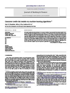
ANNs are machine-learning algorithms, based on learning from data, that are capable of solving prediction and classification problems. Multilayer perceptron (MLP) is an ANN with a specific structure and training procedure [1,6] . The main component of MLP is the formal neuron (Figure 1a), which sums the inputs and performs a transform via the activation function, which is responsible for nonlinearity. Neurons form a structure with inputs representing exploratory variables, variable numbers of hidden layers (including the activation function), and the outputs corresponding to the target variable(s). A particular MLP structure used for spatial prediction contains two input neurons for the x and y coordinates, several hidden neurons arranged in one or two layers and responsible for modeling nonlinearity, and the output neuron(s), representing target variable values (see Figure 1b). The MLP of such a structure is a universal approximator. The number of hidden neurons is subject to optimal configuration for a particular case study. In general, the complexity of the MLP must be consistent with the amount of information for training: there should be enough data to match every connection. Choosing too many hidden neurons will thus lead to overfitting (or overlearning)—the condition that occurs when MLP loses its ability to generalize the information from the samples. On the other hand, using too few hidden neurons will not provide explicit extraction of the trend, and hence some large-scale correlation will remain in the residuals, restricting further procedure.

Application of MLP requires, first, a training phase, during which the model learns the pattern from the input and output data. Training involves use of the quadratic mean square error (MSE) cost function for optimizing the summation weights at each neuron. A back-propagation error algorithm is applied to calculate the gradient of MSE on adaptive weight, E / W . Various optimization algorithms that employ back propagation can be used, such as the conjugate-gradient-descent method, the second-order pseudo-Newtonian Levenberg-Marquardt method, or the resilient propagation method [6]. After the MLP has been trained and the optimal weights have been found, spatial prediction can be computed by feeding the coordinates of the location of interest to the MLP input and reading the results from the output.

The general regression neural network (GRNN) is another type of ANN based on local kernel smoothing (kernels are placed at each data location) [6]. Assuming equal normally distributed random variables over the entire space, conditional probability is estimated with the semiparametric Nadaraya-Watson kernel method, using Gaussian kernel bandwidth as the model parameters [14,20]. Kernels are placed at the data locations, and the optimal parameter values are obtained through minimizing the MSE cost function, using a leave-one-out (cross-validation) algorithm. GRNN is capable of providing not just a point estimate (local Kanevski, Mikhail; Demyanov, Vasily; Pozdnukhov, A.; Parkin, R.; Savelieva, E.; Timonin, V.; Maignan, M., 2003: Advanced geostatistical and machine-learning models for spatial data analysis of radioactively contaminated regions. Environmental Science and Pollution Research International (Sp. Iss. SI): 137-149

3

distribution mean), but also higher-order moments—variance, skewness, kurtosis—which are important in assessing a prediction's quality and range of uncertainty. For this purpose, obtained residuals at the training points are exposed in turn to the network, so that GRNN is retrained to provide better error estimate.

Extensions of the GRNN model involve modeling both regression (conditional mean value) and conditional probability. Assuming that local distribution can be characterized by a Gaussian probability density function (pdf), we can compute function-value probabilities to be above or below some predefined levels. This assumption does not restrict GRNN regression estimates, only the probability mapping procedure. Such models are PNN. Like GRNN, PNNs are extremely attractive for decision-oriented risk mapping, as long as they preserve the capacity of fast training and relatively low preliminary expertanalysis effort (as demonstrated in decision-support mapping of Chernobyl radionuclides). A first attempt to apply GRNN to the Chernobyl fallout data was made in Kanevski [11]. PNNs can be used in classification problems as long as they can work with categorical or indicator data [18].

A radial-basis-function neural network (RBFNN) is another type of ANN, based on kernel regression. Unlike GRNN, it employs arbitrarily located kernels with varying radii, which are assigned using unsupervised learning for locating the kernel centers and defining the width for each. More details on RBFNN can be found in Haykin [6] and Bishop [1]. Application of RBFNN for analysis and modeling of Chernobyl fallout is presented in Polishuk and Kanevski [15].

2.2

Support Vector Machines

In the early 1990s, a new paradigm emerged for learning from data, called support vector machines (SVMs). They are based on statistical learning theory (SLT) [19], which establishes a solid mathematical background for dependency estimation and predictive learning from finite data sets. At first, SVM was proposed essentially for classification problems of two classes (dichotomies); later, it was generalized for multiclass classification problems and regression, as well as for estimation of probability densities.  SVM provides nonlinear and robust solutions by mapping the input space into a higher-dimensional feature space, using kernel functions, and applying linear algorithms in this space. This approach is based on the idea that if any learning algorithm is formulated specifically in terms of dot products between the training samples, then it can be applied in any space. SVM thus provides a way for computing the dot products in high-dimensional space. One way to calculate the dot products is to use a symmetric positive definite function f: X2R, known as kernels [17]. By using different kernels, we can obtain learning machines analogous to well-known architectures, such as RBFNNs and MLPs. Thus, one of the advantages of this method is that it places into one framework some of the most widely used models, such as linear and polynomial discriminating surfaces, feed-forward neural networks, or networks composed of radial basis functions. The strength of SVM is that it attempts to at once minimize both the empirical risk (error estimation for the training data) and the complexity of the model, using the formalized bounds for "complexity" defined in SLT. Unlike the Bayesian methods, based on a modeling of the probability densities of each class, SVMs focus on the marginal data (support vectors) rather than statistics such as means and variances.

Thus, an SVM for binary classification aims to distinguish data with a hyper-plane in the kernel-defined feature space. The hyper-plane is constructed to maximize the margin between data of different classes. The boundary data are support vectors. Kanevski, Mikhail; Demyanov, Vasily; Pozdnukhov, A.; Parkin, R.; Savelieva, E.; Timonin, V.; Maignan, M., 2003: Advanced geostatistical and machine-learning models for spatial data analysis of radioactively contaminated regions. Environmental Science and Pollution Research International (Sp. Iss. SI): 137-149

4

Multiclass classification can be solved by combining several binary classifiers. The simple one-against-the-rest scheme was found to work well for spatial classification problems. SVM for regression (SVR) aims to fit a hyper-plane to the data in feature space, so that data lying inside the margin of width  are not penalized and do not affect the solution. It makes the model robust and bounds its complexity.

The final SVM/SVR model is a linear combination of kernels associated with training data. Only the most important data— support vectors—have nonzero weights, thus providing faster computation.

Practical implementation of all the SVM/SVR models requires solving a quadratic programming (QP) problem. One advantage of the model (and hence the QP problem) is that it can be easily solved with a number of numerical methods; it also has a unique solution (unlike ANN). In general, SVM/SVR models were found to be powerful and flexible models, well suited for environmental spatial data analysis and modeling applications [12].

2.3

Analysis of Residuals

Spatial modeling often faces the problem of dealing with multiscale patterns in data. The presence of large-scale spatialstructure trends complicates the modeling and often poses a serious obstacle for linear-regression models. There exist several approaches for trend modeling (detrending), such as polynomial, splines, and moving window. Machine learning has proven to be an extremely efficient approach for trend removal [12]. In this approach, residuals remaining at the training points after machine-learning modeling are subject to deep analysis. Correlation between the residuals and the initial data makes it clear that the pattern was not entirely captured by the model. Exploratory spatial data analysis of the residuals allows detection and modeling of the remaining short-scale correlation structure in the residuals, if it exists.

Geostatistics provide a basic tool—variography—for spatial-correlation analysis and modeling. First attempts at sequential application of ANN and geostatistics demonstrated the feasibility and perceptiveness of the approach [9]. Further extension of these ideas provided very interesting results [4,13]. In these works, geostatistics are used not just for sequential residual modeling, but also for controlling the quality of the machine-learning model's performance.

The variogram—a measure of

spatial correlation—provides a quantitative criterion for the ranges of spatial structure modeled by machine learning in both the large-scale trend and the trend still remaining in the residuals, if any. This feature is used extensively in machine-learning detrending, because it is important (on the one hand) not to model the trend structure without sufficient detail-capturing nonlinearities, and (on the other hand) to leave enough significant spatial correlation in the residuals for further modeling. This is achieved by computing and comparing variograms for both estimates and corresponding residuals at the training points, considering machine-learning algorithms of different complexity.

2.4

Stochastic-Simulation Models

Stochastic-simulation models are an alternative approach to prediction models. Unlike the latter, stochastic simulation provides not a single point estimate, but a set of realizations that form a distribution function of the target variable at the estimated location. Realizations of a random function (in general, described by a joint probability density function) are generated with a spatial Monte Carlo model as equally probable in some sense. The similarities and dissimilarities between the realizations Kanevski, Mikhail; Demyanov, Vasily; Pozdnukhov, A.; Parkin, R.; Savelieva, E.; Timonin, V.; Maignan, M., 2003: Advanced geostatistical and machine-learning models for spatial data analysis of radioactively contaminated regions. Environmental Science and Pollution Research International (Sp. Iss. SI): 137-149

5

describe spatial variability and uncertainty. Such an approach is capable of modeling spatial variability and stochastic spatial patterns by reproducing the first (univariate global distribution) and the second (covariance or variogram) moments. An important feature of stochastic simulation is that, as conditioned by the sample data, the latter are reproduced precisely by stochastic realizations. This is the same feature that is included in geostatistical kriging models but is lacking in other kinds of interpolation models (inverse distance methods, splines, polynomial, etc.). Simulations bring valuable information for the decision-oriented mapping of pollution. Postprocessing of simulations provides probabilistic maps: maps of probabilities of the function value to be above/below some predefined decision levels. The set of spatial-pattern realizations makes possible the assessment of extreme cases at different levels of conservatism. Stationary stochastic simulations were recently applied to radioactive-pollution mapping in combination with machine-learning detrending models [13].

There are many stochastic simulation algorithms: Gaussian-based, indicator simulations, annealing, etc. One of the commonly used approaches is sequential simulation, in which every consequently simulated value is then added to the sampled (conditioned) data set to be used for simulation at every next location. Conditioning ("hard") data are precisely reproduced by construction of the simulation algorithm.

3

Chernobyl Fallout: Case-Study Results

Radioactive soil contamination caused by Chernobyl fallout features anisotropic, highly variable, and spotty spatial patterns. The multiscale character of the pattern results from numerous influencing factors: the source term, atmospheric precipitation, weather conditions, dry and damp precipitation, surface properties (orography, ground cover, soil types, land use, etc.). The most prominent influence on long-term contamination was the radionuclide cesium (137Cs), the presence of which in the emission is a function of the source character (reactor type). The half-life of this isotope is about 30 years. The

137

Cs surface-

contamination pattern is quite spotty, highly variable, and includes outlying sample values. The monitoring network used for the sampling is often clustered—as a rule, there are more samples in the high-value areas than in the low-value areas. Such preferential sampling can lead to serious biases in estimating global characteristics of the distribution (mean, variance, etc). Thus, declustering is necessary to take into account higher the sampling density in the hot spots. Various declustering techniques exist, such as random selection and weighting. Cell declustering is usually performed in geostatistics for this purpose [5]. It allows taking into account all the available data, with the weights corresponding to the sampling density in the local neighborhood (rectangular cell). The selected region is a rectangle covering 7,428 km2 with 845 populated sites (340 in Russia and 505 in Belarus). It includes three administrative divisions: Gomel (three districts, 83 populated sites), Mogilev (four districts, 422 populated sites), and Briansk (four districts, 340 populated sites). The measurements (including probes taken at different times around each populated site) were collected at the sites and then averaged, with weighting based on expert opinion. The single data value corresponding to the given location is the contamination density in kBq/m2, recalculated to the fixed time of the initial fallout, April 1986. These data from 684 locations were considered as the "hard" samples of the target variable,

137

Cs. (See the data

post plot in Figure 2a.) Also, important additional "soft" information about the Chernobyl fallout can be rigorously incorporated into the prediction-mapping framework and can lead to significant improvement of the results. The minimum and maximum probe values available at the sampling locations define the range of the random function distribution at the point. A number of probes used to calculate the averaged "hard" value provides a confidence level for each location, which, along with Kanevski, Mikhail; Demyanov, Vasily; Pozdnukhov, A.; Parkin, R.; Savelieva, E.; Timonin, V.; Maignan, M., 2003: Advanced geostatistical and machine-learning models for spatial data analysis of radioactively contaminated regions. Environmental Science and Pollution Research International (Sp. Iss. SI): 137-149

6

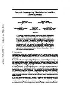
the size of the populated site, was used by the expert sampling uncertainty criterion. Data were split into training and testing sets for the purpose of controlling the machine-learning process and final-prediction quality assessment. Testing data were selected at random from local rectangular cells with respect to monitoring network clustering. The similarity of global statistics and spatial correlation of the training and test data were the main criteria for splitting the data into the two sets. The locations of the points from both data sets are shown in Figure 2b. The spatial correlation structure of 137Cs contamination in the selected region features significant trends, visible in Figure 2a as a decreasing tendency, especially strong in the east direction. One of the quantitative measures of spatial trend is drift function: D(h) = E[Z(x) – Z(x + h)]

,

(1)

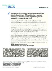
where Z(x) and Z(x + h) represents a pair of values separated by vector h. Drift for 137Cs computed for different directions of h is presented in Figure 3a. The anisotropic character of the drift is clearly shown in Figure 3b. Such complex behavior is one reason to apply nonlinear trend machine-learning models.

4

Modeling Results and Discussion

4.1

Multilayer Perceptron (MLP) Prediction Mapping Using Additional Information

MLP models of varying architectures were applied to

137

Cs for two reasons: (1) to model long-range nonlinear trends to

facilitate further geostatistical modeling of the residuals; and (2) to make the best possible prediction with the MLP model, using only additional available information on sampling destitution and uncertainty. The trend-modeling task was successfully executed with a simple MLP 2-5-1, with five neurons in a single hidden layer. This number of neurons was enough to capture long-range nonlinearity while leaving enough correlated information in the residuals (see Figure 5b). Gridded trend estimates are presented in Figure 6a. Geostatistical spatial correlation analysis was used to control the quality of the MLP performance through the variogram—a basic geostatistical measure of spatial continuity. A semi-variogram (or variogram) is defined as a variance of increments between the function values separated by vector h: γ(h) = ½Var[Z(x + h) – Z(x)] .

(2)

Variograms are used intensively in geostatistical regression models (kriging) to model spatial correlation, taking into account anisotropy. In our case, variograms plotted for the raw data, MLP estimates, and the corresponding residuals at the training points (see Figure 4) show evidence of trend and multiscale structure variogram exceeds the a priori data variance); the MLP estimates capture long-scale correlation up to 30 km; and the remaining residuals feature stationary behavior (the variogram levels off at a constant value) in the 12–15 km range. Thus, MLP modeled long-scale spatial nonlinearity well and allowed the variogram for the residuals to reproduce the original data correlation very closely over a short range.


7

MLPs of more complex structures—two hidden layers and more neurons—were applied to prediction mapping. Given a significant amount of data (484 training locations), the number of neurons was increased. MLPs with two hidden layers (each with 10 neurons [2-10-10] and 8 and 5 neurons [2-8-5]) provide from 1.5 to 7.0 data points per network connection, which means that a very thorough and detailed level of modeling is expected. Two kinds of outputs were considered. First, we considered a conventional single output corresponding to the average

137

Cs data as applied in the above simple MLP (see

Figure 6b). Then, an MLP with 3 output neurons was considered, to take into account additional information from the minimum and maximum sample values available at each training point (see Figure 7). Minimum and maximum probes provide the local distribution range for every sampling location, contributing to rigorous uncertainty assessment and improvement of overall prediction quality. Also, additional information on the number of probes used to obtain each averaged datum was incorporated as the training weights in a minimization algorithm. This implies that more probes would provide more confidence to the average data value. The quality of MLP performance was checked on the test data by comparing basic statistics (mean and standard deviation) and the correlation of the estimates to the measurements at the testing locations (see Figure 5a). These results are summarized in Tables 1 and 2. Residuals remaining after modeling with more sophisticated MLPs are not correlated, unlike the ones for a simple MLP structure of 2-5-1 (see Figure 5b). Comparing MLPs of the same complexity, the ones with three outputs give smaller mean square error (MSE) and higher correlation with the test data, which indicates their higher generalization ability. MLP 2-8-5-3 is best in terms of matching the mean and standard deviation of the overall global data distribution.

4.2

General Regression Neural Network (GRNN) Prediction and Risk Mapping

GRNN was applied to 137Cs contamination data to provide spatial predictions accompanied by estimation errors (see Figure 8). GRNN with one output (137Cs average) and three outputs (137Cs min/max/aver) were compared. There appeared to be little difference between the estimates provided by the single-output and the three-output networks. However, the estimation errors show some difference. GRNN using additional data on the minimum and maximum provides more realistic confidence intervals than the one based only on the averaged samples. Thus, 86 out of 200 test data fall within the 2 interval for threeoutput GRNN, while only 76 fall within this interval for single-output GRNN. Moreover, the estimation error provided by GRNN still seems to underestimate the real variance. However, the quality of GRNN estimates is as good as the best MLP predictions in terms of testing MSE and correlation with the test data. GRNN is able to capture almost the entire spatial structure over both long and short scales, leaving no significant correlation in the residuals, so they are not suitable for further modeling. Another advantage of GRNN is that it can provide an estimate for the probability that the

137

Cs concentration will

2

exceed a certain level (800 kBq/m ). Such risk maps are extremely valuable for decision making (see Figure 9).

4.3

SVR Prediction Mapping

The case study of predictive spatial mapping using support vector regression (SVR) follows the general methodology of spatial data analysis with geostatistics and machine-learning algorithms. The detailed description of this case study that explains basic SVR and extended SVR methods can be found in Kanevski et al. (2002). The data were split into training, testing, and validation subsets. The most important phase of the modeling is selection of the optimal SVR hyper-parameters. Several hyper-parameters have to be selected for SVR modeling: , C, and kernel parameters. The kernel choice is an important part of the SVR application. A Gaussian RBF kernel was found to be the most suitable because it is easy to interpret, Kanevski, Mikhail; Demyanov, Vasily; Pozdnukhov, A.; Parkin, R.; Savelieva, E.; Timonin, V.; Maignan, M., 2003: Advanced geostatistical and machine-learning models for spatial data analysis of radioactively contaminated regions. Environmental Science and Pollution Research International (Sp. Iss. SI): 137-149

8

has one free parameter—bandwidth—and it is often used in other machine-language methods. All these features make the Gaussian RBF kernel attractive for spatial data mapping. Isotropic RBF kernels were used for the present case study. In this case, given L training locations xi we seek the regression function f(x) in the form: L

f ( x)   i e



x  xi 2 2

2

b

,

(3)

i 1

where  is the kernel bandwidth predefined by user, and weights i and the threshold b are the parameters to optimize. The common methods for tuning the parameters in machine-language algorithms are cross-validation (or K-fold cross-validation) and calculation of testing error on some subset of the entire dataset. A comprehensive search in 3D hyper-parameter space (, , C) was performed. Some 2D error surfaces (, C) are presented in Figure 10. For the numerical stability of the algorithm, 137

Cs activity values were scaled linearly into the [0,1] interval. The value of the  parameter was fixed at  = 0.02.

As can be seen, the solution is more sensitive to kernel bandwidth than to C. In general, the following conclusions were made about parameter influence on the model: —kernel bandwidth. The most evident properties depending on this parameter occur at small  values—much less than the region's area—where the model is close to overfitting; and at large  values—of the order of the region's area—where the model is close to oversmoothing (or underfitting, in machine-learning terminology). The same is clear from the SLT side: small  values lead to a very powerful model in a too-high dimensional space—too many features are used for modeling, which leads to overfitting. The optimal value of this parameter depends primarily on two data characteristics: correlation radius and data variability. In general, the question of optimal sigma is connected with the complicated question of monitoring network analysis: whether we can describe given/unknown phenomena with the measurements from a given monitoring network.

C—the parameter that defines the tradeoff between training error and model complexity; an inverse value is the regularization constant. This parameter defines the upper bound of the multipliers i; hence, it defines the maximal influence that the point can exert on the solution. —the width of the insensitive region of the loss function. This parameter defines the sparseness of the SVR solution: the points that lie inside the -tube have zero weights. It is the main parameter incorporating information on measurement quality. It is possible to set values of  and C individually for every point, using some additional information on measurement quality, confidence measures, etc. The following parameters were selected for modeling: C = 0.32,  = 0.02, and  = 4. This SVR model was applied to the validation data, a part of the data not used for training/tuning of the model. The following results were obtained: training error 0.048, testing error 0.071, validation error 0.064, and correlation coefficient between validation data and its prediction by the model, 0.86. The results of prediction mapping are presented in Figure 11.


9

Modeling results were controlled using exploratory variography of the residuals on validation data. The variogram demonstrated an almost pure nugget effect; hence, all the spatially structured information had been extracted by the model.

4.4

Uncertainty Modeling of the Residuals with Stochastic Simulations

Residuals obtained after detrending with machine-learning algorithms were used for further modeling. After a nonlinear, longscale trend has been removed with a simple MLP 2-5-1, the remaining residuals feature stationary behavior. A stationary variogram model was built and fitted for normalized residuals in order to run sequential Gaussian simulations (SGS). However, normalization of the residuals does not imply assumption of their Gaussian distribution, as normal score transformation is made to reduce the influence of outliers. Also, sequential stochastic simulation of normalized variables ensures correct reproduction of the global distribution along with spatial statistics. Fifty equally probable stochastic realizations of the residual spatial distribution were computed using the SGS algorithm. Each of them preserves the histogram and the variogram of the original distribution.

The final result is delivered as the sum of the MLP trend estimate and the SGSIM simulated residual. The mean of the simulated values at each location can provide an averaged map of estimates (see Figure 12a), but this is not the strongest output of the model. The uncertainty is fairly realistically quantified by the difference between the simulated patterns characterized by standard deviations of the local distributions at each simulated node (see Figure 12b). The local distribution function can be fairly realistically described, given the set of values at each node. Obtaining the local distribution of the realizations again at the testing points, we checked the original measurements, respecting the confidence intervals determined by standard deviations of the local distributions. Thus, out of 200 test data, 190 fall into the 2 confidence interval, which is, for example, twice as good as the result given by confidence intervals for GRNN predictions. Furthermore, based on the local distribution function, it is possible to derive the probability of exceeding a certain level of concentration. The map of probability for

137

Cs to exceed the level 800 kBq/m2 is presented in Figure 13. It is obviously smoother than the one provided

by GRNN.

4.5

Classification with SVM, KNN, and PNN

The contemporary models for analysis of spatially distributed categorical data are presented in this chapter: SVM and PNN. The methods are compared to the traditional nonparametric k-Nearest Neighbor classifier by using independent validation data sets. Gaussian RBF functions were used as SVM kernels. A one-against-the-rest scheme was used for M-class classification: M binary classifiers are trained; each of them classifies one of the classes against all other classes. Then the classes are combined into one M-class classifier: the point is assigned to the class that has the highest output. The model is quite flexible, since we can vary the parameters of each binary classifier to take into account different spatial variability of classes.

PNN is a supervised neural network used widely in the field of statistical pattern recognition and the estimation of classmembership probability. PNN uses a Bayesian optimal (or a maximum posterior) decision rule. The model uses nonparametric density estimation, based on a kernel approach, and is a direct implementation of the kernel-based pdf estimator and Bayesian decision rule. Note that a traditional geostatistical approach for classification—indicator kriging—may fail, since it requires modeling of the spatial correlation structure of the classes, which can be impractical for lack of data. Kanevski, Mikhail; Demyanov, Vasily; Pozdnukhov, A.; Parkin, R.; Savelieva, E.; Timonin, V.; Maignan, M., 2003: Advanced geostatistical and machine-learning models for spatial data analysis of radioactively contaminated regions. Environmental Science and Pollution Research International (Sp. Iss. SI): 137-149

10

The real case study deals with the problem of soil-type classification in the Bryansk region, the most contaminated region in Russia after the Chernobyl accident. This task is of special importance, since radionuclide migration over time and space depends critically on soil type, and this dependence influences prediction mapping of contamination and dose estimates. Five soil types/classes (loam—Class 1, sandy—Class 2, sandy-swamped—Class 3, clay—Class 4, and sandy-loam—Class 5) exist in this region. The original data set contains 810 sample points (the monitoring network for radionuclide concentration). It was split into two parts: training and validation data subsets. Original geographic coordinates were first transformed to metric Lambert map projection and then linearly projected to the (–1; 1) segment for numerical stability of the algorithms. The training data set is used to train models to adjusted weights. It contains 310 samples homogeneously distributed over the region. A validation data set is used to check and to compare obtained results; it contains the remaining 500 samples. The data are presented in Figure 14. Parameters of the models were tuned by cross-validation error minimization. The results of prediction mapping are presented in Figure 15. Validation results are presented in Table 3.

All the models performed quite well, but the validation results for classification of different classes differ. For example, the error for Class 4 is 60%, because of the insufficient amount of training data in this class. It was also found that the methods represent the spatial structure of major classes. Note also that SVM gives a hard decision boundary, whereas PNN provides the probability of belonging to a class. Details on SVM and PNN application for spatial classification of the Chernobyl fallout data can be found in Pozdnukhov et al. [16]. 5

Conclusions

This paper presents a review of the most recent advances in spatial data analysis and modeling of the Chernobyl fallout data and associated problems. The work covers application of the recently developed machine-learning algorithms, together with existing geostatistical and stochastic simulation models. In our study, many machine-learning algorithms now currently used for data mining purposes (MLP, GRNN, PNN, RBFNN, SVM/SVR) demonstrate their excellent applicability to Chernobyl radioactive fallout issues (with model performance comparisons based on training and testing data sets). 

ANNs were able to take into account additional information on sampling distribution, which allowed for improved prediction quality and estimation of confidence.



MLP algorithms demonstrated their strength, both in modeling nonlinear long-scale trends and in providing fair prediction. Particular efficiency was achieved by using geostatistical analysis for controlling quality of machine-language results and further modeling of the residuals.



Stochastic simulations applied in combination with MLP detrending provided realistic uncertainty assessments and risk mapping for 137Cs contamination—particularly valuable for decision-making support.



SVM, used for soil type classification, demonstrated efficient multiclass spatial-data classification. It delivered better results than PNN and nearest-neighbor models.



PNN provided very important additional information: probabilistic modeling (class probabilities). It can be used for description of classification uncertainty. Also, PNN enables taking into account a priori information.

The application of machine-learning modeling enhanced results when applied to the Chernobyl data. Machine-learning methods usually require a sufficient amount of data to train on and, fortunately, existing Chernobyl databases provided a needed amount of information to be integrated into the modeling framework. A conventional geostatistical analysis solely Kanevski, Mikhail; Demyanov, Vasily; Pozdnukhov, A.; Parkin, R.; Savelieva, E.; Timonin, V.; Maignan, M., 2003: Advanced geostatistical and machine-learning models for spatial data analysis of radioactively contaminated regions. Environmental Science and Pollution Research International (Sp. Iss. SI): 137-149

11

applied to the Chernobyl data had suffered from complex spatial-correlation modeling due to multiscale nonstationary patterns. Incorporating machine-learning models solved detrending problems in such complicated cases and eased consequent geostatistical modeling.

Acknowledgments

The work described here was supported in part by CRDF grant RG2-2236, INTAS Grants 99-00099, 97-31726, INTAS Aral Sea Project #72, and Russian Academy of Sciences Grant for Young Scientists Research #84, 1999. The authors thank S. Chernov for programming GEOSTAT OFFICE software, which was extensively used in the research.

References

[1] Bishop CM (1995): Neural Networks for Pattern Recognition. Oxford, Clarendon Press [2] Cressie N (1991): Statistics for Spatial Data. John Wiley & Sons, New York, 900 pp [3] De Cort M, Tsaturov Yu S (1996): Atlas on Caesium Contamination of Europe after the Chernobyl Nuclear Plant Accident. European Commission, report EUR 16542 EN, 39 pp [4] Demyanov V, Soltani S, Kanevski M, Canu S, Maignan M, Savelieva E, Timonin V, Pisarenko V (2001): Wavelet analysis residual kriging vs. neural network residual kriging, Springer, Stochastic Environmental Research and Risk Assessment, 15 (1)18–32 [5] Deutsch CV, Journel AG (1998). GSLIB Geostatistical Software Library and User's Guide. Oxford University Press, New York, Oxford [6] Haykin S (1999): Neural Networks. A Comprehensive Foundation. Second Edition. Prentice Hall International, Inc. [7] Israel YA, Kvasnikova EV, Nazarov IM, Stukin ED, Fridman ShD (1997): Atlas of radioactive contamination of European Russia, Belarus and Ukrainet. Possibilities and perspectives of development. 18th ICA/ACI, ICC'97 Proceedings, Ed. L Ottson, 2 pp 646–653 [8] Kanevsky M, Arutyunyan R, Bolshov L, Demyanov V, Maignan M (1996): Artificial neural networks and spatial estimations of Chernobyl fallout. Geoinformatics, 7 (1–2) 5–11 [9] Kanevsky M, Arutyunyan R, Bolshov L, Demyanov V, Linge I, Savelieva E, Shershakov V, Haas T, Maignan M (1996): Geostatistical Portrayal of the Chernobyl Fallout. Geostatistics Wollongong '96, Ed. EY Baafi, N Schofield, Kluwer Academic Publishers, Vol. 2, pp 1043–1054 [10] Kanevsky M, Arutyunyan R, Bolshov L, Chernov S, Demyanov V, Linge I, Koptelova N, Savelieva E, Haas T, Maignan M (1997): Chernobyl Fallouts: Review of Advanced Spatial Data Analysis. geoENV I – Geostatistics for Environmental Applications, Ed. A Soares, J Gomez-Hernandes, R Froidvaux, Kluwer Academic Publishers, pp 389–400 [11] Kanevski MF (1998): Spatial predictions of soil contamination using general regression neural networks. Intern. J. Systems Research and Informational Science, 8 241–256 [12] Kanevski M, Pozdnoukhov A, Canu S, Maignan M. (2002): Advanced Spatial Data Analysis and Modelling with Support Vector Machines. International Journal of Fuzzy Systems, 4 (1) 606–616 [13] Kanevski M, Parkin R, Pozdnukhov A, Timonin V, Maignan M, Demyanov V, Canu S (2003): Environmental Data Mining and Modelling Based on Machine Learning Algorithms and Geostatistics. Environmental Modeling and Software, Elsevier, accepted Kanevski, Mikhail; Demyanov, Vasily; Pozdnukhov, A.; Parkin, R.; Savelieva, E.; Timonin, V.; Maignan, M., 2003: Advanced geostatistical and machine-learning models for spatial data analysis of radioactively contaminated regions. Environmental Science and Pollution Research International (Sp. Iss. SI): 137-149

12

[14] Nadaraya EA (1964): On estimating regression. Theory of Probability and its Applications, 9 141–142 [15] Polishuk V, Kanevski M (2000): Comparison of unsupervised and supervised training of RBF neural networks. case study: Mapping of contamination data, Proceedings of the Second ICSC Symposium on Neural Computation (NC'2000), Berlin, Germany, pp 641–646 [16] Pozdnukhov A, Timonin V, Kanevski M, Savelieva E, Chernov S (2002): Classification of Environmental Data with Kernel Based Algorithms. Preprint IBRAE-2002-09, Moscow: Nuclear Safety Institute RAS, 22 pp [17] Scholkopf B, Smola A (2002): Learning with Kernels, MIT press [18] Specht D (1990): Probabilistic neural networks. Neural Networks, 3 109–118 [19] Vapnik V (1998): Statistical Learning Theory, John Wiley & Sons [20] Watson GS (1964): Smooth regression analysis. Sankhya: The Indian Journal of Statistics, Series A, 26 359–372


13

w0 w1 w2 . . .

 x

wn Inner Production

f Activation Function

(a)

(b)

Figure 1: Formal neuron (a) MLP with two inputs, as well as five hidden and three output neurons


14

a)

b) Figure 2. Raw data on

137

Cs concentration in the Bryansk region a), locations of the training and the testing points

b).

a)

b)

Figure 3. The drift of 137Cs data: (a) directional (degree clockwise from horizontal); (b) 2D rose diagram


15

Figure 4. Omnidirectional variograms for raw data MLP 2-5-1 estimates and the remaining residuals

a)


16

b) Figure 5. Scatterplot of MLP results : (a) estimates vs. the measurements at the testing locations for three different architectures: 2-5-1, 2-10-10-1, and 2-10-10-3; (b) residuals vs. the measurements at the training points for MLP 2-5-1 and 2-10-10-3.

a)

b) Figure 6.

137

Cs estimates: (a) long-range trend with MLP 2-5-1; MLP 2-10-10-1 with a single output (b)


17

a)

b)

Figure 7. MLP estimates of 137Cs: (a) MLP 2-8-5-3 and (b) MLP2-10-10-3, with three outputs corresponding to average/minimum/maximum 137Cs samples.

a)

b) Figure 8. GRNN modeling of 137Cs contamination: a) estimates and b) estimation error.


18

Figure 9. Probability of 137Cs concentration to exceed the level of 800 kBq/m2 obtained with GRNN.

a)

b)

Figure 10. (a) Training and (b) testing error surfaces


19

Figure 11. 137Cs estimates with SVR

a)

b)

Figure 12. Neural network residuals sequential Gaussian simulations (NNRSGS): (a) mean estimate and (b) standard deviation for 50 realizations


20

Figure 13. Probability of 137Cs concentration to exceed the level of 800 kBq/m2 obtained with NNRSGS model

a)

b)

Figure 14. Data on soil-type classes: (a) at the training locations and (b) at the testing location, with Voronoi polygons used for visualization.

a)

b)


21

Figure 15. Categorical prediction mapping of soil types with (a) SVM and (b) PNN Table 1: Mean square errors (MSE) and correlation coefficients (o) for prediction of training and testing data sets

MLP structure

Correlation 0

MSE Test set

Training set

Test set

Training set

2-5-1

179,426

194,177

0.612

0.638

2-10-1

100,322

113,119

0.812

0.809

2-8-5-1

105,686

89,047

0.797

0.863

2-10-10-1

87,924

46,469

0.838

0.932

2-8-5-3

107,346

69,490

0.806

0.888

2-10-10-3

77,602

75,567

0.853

0.881

2-8-5-3 w/ weights

127,358

80,840

0.763

0.868

2-10-10-3 w/ weights

109,352

66,648

0.815

0.893

Table 2: Comparison of statistics for different models MLP structure

Mean

Std. deviation

Testing data set

554

533

All data

572

562

2-5-1

560

372

2-8-5-1

524

462

2-10-10-1

549

507

2-8-5-3

579

518

2-10-10-3

546

470

2-8-5-3 w/ weights

568

501

2-10-10-3 w/ weights

589

550


22

Table 3: Validation results of the classification models Soil classes

SVM

PNN

k-NN

Misclassified

%

Misclassified

%

Misclassified

%

All classes

64

12.8

91

18.2

89

17.8

Class 1 Loam

18

13.4

23

17.2

23

17.2

Class 2 Sand

0

0

2

13.3

2

13.3

Class 3 Sandy-swamped

14

10.7

28

21.4

25

19.1

Class 4 Clay

15

60

12

48

15

60

Class 5 Sandy-loam

17

8.7

26

13.3

24

12.3


23