The requirements on the GNC systems for these missions are very ... The GNC system is based on advanced algorithms, and low-cost, off-the-shelf actuators ...
6TH EUROPEAN CONFERENCE FOR AERONAUTICS AND SPACE SCIENCES (EUCASS)
Advanced vision-based navigation for approach and proximity operations in missions to small bodies Kicman, P.*, Gil, J.**, Lisowski, J.*** and Bidaux-Sokolowski, A.*** * GMV, Marie Sklodowska-Curie fellow ** GMV, S.A. Tres Cantos, Spain *** GMV Innovating Solutions, Sp. z o.o. Warsaw, Poland
Abstract The paper presents vision-based navigation system for descent and landing (D&L) on Phobos. The investigated technique is called Enhanced Relative Navigation (ERN) and is a method based on landmark matching to calculate the position of the spacecraft with respect to the surface. Various types of feature extractors and descriptors are evaluated on rendered images (7.68m accuracy) and on images of an asteroid mock-up obtained in GMV’s platform-art laboratory (10.9m accuracy). The algorithm is able to successfully recognize and match landmarks in the presence of substantial changes of viewing angle and under varying illumination conditions. Recommendations are provided in order to increase method robustness and advance its TRL.
1. Introduction Robotic exploration missions to small bodies require advanced technologies, especially a sophisticated Guidance, Navigation & Control (GNC) techniques. The requirements on the GNC systems for these missions are very demanding. Cost shall be minimized, reducing the sensor suite and in the same time tight orbital and landing performances have to be fulfilled. Furthermore, robustness is a fundamental concern because of the high level of uncertainty of the environment. An autonomous GNC system for descent and landing (D&L) on Phobos is being developed by GMV under ESA contract. The GNC system is based on advanced algorithms, and low-cost, off-the-shelf actuators and navigation sensors with high Technology Readiness Level (TRL). Presented study builds on top of previous projects done by GMV for ESA, mainly MarcoPolo-R and NEO-GNC. The GNC system includes two different vision-based navigation strategies: pure Relative Navigation (RN) and Enhanced Relative Navigation (ERN). Both strategies are based on the tracking of unknown features on the surface of the asteroid. The differences are mainly in the initialization procedures. Focus of the presented study is placed on the visual navigation algorithms that can increase the autonomy of the GNC system, reduce navigation errors and reduce mission costs in terms of ∆V. In the paper, we are presenting an absolute navigation method, based purely on image processing that allows accurate calculation of the spacecraft position with reference to the target body.
2. Vision-based navigation The core of the navigation system consists of the relative navigation algorithm based on unknown feature tracking and supported by altimeter measurements. Details and performance results of the RN algorithm have been provided in [10]. The architecture of the system extended by ERN algorithm is shown in Figure 1.
Copyright 2015 by Kicman, P, Gil. J., Lisowski, J., Bidaux-Sokolowski, A.. Published by the EUCASS association with permission.
Kicman, P., Gil, J., Lisowski, J., Bidaux-Sokolowski, A.
Figure 1. Navigation system architecture. To increase the autonomy and accuracy of the system we propose an Enhanced Relative Navigation method. In essence it is the same RN algorithm that can be autonomously initialized by means of landmark recognition on the surface of the target body and computing initial position of the spacecraft. The improvement of the navigation performances comes from better initialization of the navigation filter and reduced impact of a priori ground-provided knowledge (orbit prediction, Phobos/asteroid rotational state). These two measures avoid time propagation of initial uncertainties since last ground update and increase the robustness to other uncertainties or off-nominal conditions. In this implementation a landmark recognition algorithm is used only to initialize the descent sequence and the navigation filter. Then, only pure relative navigation is used in the entire D&L phase. The use of Enhanced Relative Navigation offers the following simplifications and advantages in comparison to the full Absolute Navigation approach: Only a reduced set of landmarks in the neighborhood of the landing site is used (reduces significantly the matching space and number of possible combinations). Landmark recognition is performed in conditions similar to the landmark database generation – similar resolution and illumination conditions can be ensured. Close initial guess provided by navigation filter improves robustness and convergence of the algorithm. Known landmark identification algorithm is NOT in the critical operational GNC chain (GNC is always based on relative navigation). Thus, there is no time constraint and the SC can wait many GNC cycles for a successful detection. Fact that ERN is not in main GNC chain allows for confirmation of the solution by the ground while SC is waiting in body fixed hovering. Lack of strict time constraints enables also calculation of additional checks onboard to ensure correctness of the solution. Initial step of the algorithm is a landmark database generation. Then, the database is uploaded to the SC and used for position calculation. Details on the database generation procedure are given in chapter 2.1. Chapter 2.2. contains information on the landmark matching and position calculation algorithms and in chapter 3. we present the results of the preliminary algorithm verification.
2.1. Database Generation An essential part of performing landmark recognition is a generation of a database that contains information about robust landmarks. In general the database shall be built for several altitudes above the landing site because the level of details observable on different heights differs significantly. In case of ERN this process is simplified as a database only for one specific altitude is generated. It is created using images collected during characterization phase as well
2
ADVANCED VISION-BASED NAVIGATION FOR APPROACH AND PROXIMITY OPERATIONS IN MISSIONS TO SMALL BODIES
as during the close fly-bys. As the images should have a similar resolution to the one achieved by navigation camera at hovering altitude, the ground resolution of the images should be adjusted accordingly. The database is generated automatically and the process can be divided in two main steps (Figure 2): Generation of development database (db_dev) Database consolidation (db_cons) Such high-level division gives several advantages. First of all it takes into account the real process of generating database. During the mission, new images will be available with time. The development version of the database has an open structure that allows accommodation of new images at any time. On the other hand, the consolidated database is a concise compilation of the development database. It is meant to be uploaded to the spacecraft and its only purpose is to be used for efficient position calculation. Another advantage of having the development version of the database is that it can be investigated and corrected by a human supervisor if such need arises. The individual steps of the algorithm are described in detail in the following paragraphs.
Figure 2. High-level view of database generation procedure.
2.1.1. Image to image matching As the first step of the algorithm, the point features are extracted from the images along with the descriptor vectors. For the purpose of this paper, several different combinations of feature extractors and descriptors have been tested (for details see Table 1). To ensure an even spread of features in the entire image the photograph is divided into an 8x8 grid and limited number of points is being retained in each grid cell. The features are stored in a convenient structure that allows easy identification of the image in which they were detected. The numbering convention for all detected features is noted in the Figure 3. Table 1. Combinations of feature extractors and descriptors used for the tests. Feature Symbol KLT_H + ORB
KLT_H + BRISK KLT_H + SIFT KLT_H + SURF SURF
KLT_S + ORB
Description KLT_H is a hardware, fixed-point implementation of KLT [1] algorithm that is limited to detecting and tracking 100 corners at each image. ORB is a binary feature descriptor [2] KLT_H combined with binary feature descriptor BRISK [3] KLT_H combined with SIFT feature descriptor [4] KLT_H combined with SURF feature descriptor [5] It is a software implementation of SURF [5] feature detector and descriptor provided in OpenCV [6] library. The amount of detected features is limited to 400. KLT_S is an OpenCV implementation of KLT algorithm. Number of features in each image is limited to 400.
Once all features are extracted, the images are compared to each other in everyone-to-everyone fashion, which means the growth of process computation complexity is quadratic with the number of available images. However, because the database generation is to be performed on the ground, time constraints are not the critical aspect of this operation. The features are matched using brute force matching procedure. It means that the distances between all descriptors are calculated and the two points that have shortest distance to each other are considered to be matches. For binary
3
Kicman, P., Gil, J., Lisowski, J., Bidaux-Sokolowski, A.
descriptor (ORB and BRISK) the Hamming distance is used as the measurement metric. For SURF and SIFT, the Euclidean distance is used. An example of points matched between two different images is given in Figure 4. I1 F1
F2
I2 …
FM1
F1
F2
…
I3 …
FM2
F1
F2
…
FM3
F1
F2
IN-1 …
FMN-1
F1
F2
IN …
FMN
Figure 3. Numbering convention for detected features. Note that number of features detected in each image can differ.
Figure 4. Features matched between two images of the same area.
2.1.2. Graph of interconnections Based on all detected features an adjacency matrix (Figure 5) is formed. It represents an undirected graph which stores in convenient way the information about matches between the features. Each column and row correspond to interconnections detected between a features detected in a particular image (i.e. I 1F2, means second feature detected in the first image). The adjacency matrix is stored in computer memory as a sparse logical array. Whenever a match is detected the value in appropriate matrix cell is set to 1 (green fields in Figure 5). At this point, database has still an open architecture and whenever new images are available they can be easily added to the existing structures. I1,F1 I1,F1 I1,F2 I1,F3 … IN,FM-1 IN,FM
I1,F2
I1,F3
…
IN,FM-1
IN,FM
X X X X X X
Figure 5. Adjacency matrix stores information about connections between all detected features. As a first step to generating consolidated database, an analysis of interconnected components is performed. Each potential landmark is represented within a graph as a set of connected features that are matched with each other, but not with other elements of the graph. The performed procedure detects each independent region of the graph, in practice dividing it into a set of smaller subgraphs. Every subgraph represents individual landmark candidate. To ensure that only the most robust landmarks are used the graphs are tested for connection strength. The maximum number of possible connections between nodes in a
4
ADVANCED VISION-BASED NAVIGATION FOR APPROACH AND PROXIMITY OPERATIONS IN MISSIONS TO SMALL BODIES
graph is equal to k k 1 , where k is the number of nodes. More connections between each feature occurrence means that the potential landmark was successfully recognized and matched in many images (Figure 6, left). This means that the point is well observable under different viewing angles and changing lighting conditions. If not enough interconnections are detected (in our case less than 50% of all possible interconnections) the landmark is rejected as not robust enough (Figure 6, right). 2.5 5
2
4 3
1.5
2
1 1
0.5
0 -1
0 -2
-0.5 -3 -4
-1
-5
-1.5 -2
-1.5
-1
-0.5
0
0.5
1
1.5
-5
2
-4
-3
-2
-1
0
1
2
3
4
5
Figure 6. Visualization of interconnections between nodes of a landmark graph. Left: robust landmark - many interconnections; Right: poor landmark, little interconnections.
2.1.3. Extraction of robust landmarks After the robust landmarks are identified, they are further processed into the form that can be used for absolute navigation onboard a spacecraft. At first the features are triangulated to compute the 3D position of points. Since the position of the camera at the point when images were taken is assumed to be known this process is straightforward. The position is calculated with a textbook nonlinear triangulation algorithm given in [7]. The points that are triangulated with the highest residual position are rejected, as it usually means that they are contaminated by outliers. At this point, the consolidated database shall contain only robust landmarks that passed all the tests and outlier detection procedures performed so far. The last operation that is performed is re-computation of the landmark descriptor. Each landmark is described by a set of descriptors, one for each point detected in images and associated with given landmark. In case of the floating point descriptor (SIFT and SURF), the landmark descriptor is simply computed as the mean value of all descriptors contributing to the landmark. The standard deviation is also stored to enhance the landmark identification process. For binary descriptors (ORB and BRISK) each value in the landmark descriptor vector is set to 1 if most (50% or more) of the points have a value at this position equal to 1, and 0 in the opposite case.
2.2 Landmark identification and position computation The same feature detection procedure is used as the one for database generation. When the features are detected, their descriptors desci are compared with the database descriptors desc j , to find the best matches. Again, the brute-
force matching procedure is performed. However, to accommodate for the uncertainties in the landmark descriptor, the uncertainty of the descriptor is used as a weight vector for distance d ij computation:
d ij2 desci desc j V j where
1
desc
i
desc j
T
(1)
V j is a diagonal matrix with landmark j descriptor standard deviation of the on the diagonal. This process is
performed only for the Euclidean distance calculation for floating point descriptors. The binary descriptors are compared using standard Hamming distance metric (eq. 2), which indicates how many elements of two binary vectors are not identical (the more different elements, the higher the distance). The Hamming distance is in the range between 0 and 1, where 0 means two identical vectors and 1 is a result for a binary vector and its negation (i is a feature index, j is a landmark index, k is an index of element within the descriptor and n is a length of the descriptor vector).
5
Kicman, P., Gil, J., Lisowski, J., Bidaux-Sokolowski, A.
dij # desci [k ] desc j [k ] n
(2)
Once the detected points in the image are matched with the database we have a set of 2D points and corresponding 3D coordinates of landmarks. Computation of camera position from such data is called in computer vision PnP problem. To solve it at least 4 valid matches are required. One of the most effective algorithms reported in recent years is the EPnP algorithm [8]. It was also used in presented experiments.
3. Algorithm testing To evaluate the performance of the algorithm a tests are performed on both simulated and real images. Separate set of images is used for generation of database and evaluation of the position calculation algorithm. Images used for database generation are captured in a circular pattern, executed at constant altitude, with camera constantly directed towards the same point (i.e. landing site). Images are taken with 10° of angular separation on the circle, which gives 36 images for full circle. The camera has 20° FOV and the image resolution is 1024x1024 pixels. As a testing set a series of 100 images is used. They were captured at the same altitude as the photographs used for database generation, however at a positon directly above the landing site. So in this case the viewing angle between images used to generate database and the test images is around 11°. The illumination conditions are similar to those at which database images were captured; however in this case movement of Sun is also simulated. Sample test images from both datasets are given in Figure 7. Simulated images are rendered with PANGU (Planet and Asteroid Natural Scene Generation Utility) 3.30 [9], a tool used for generation of realistic images of celestial bodies. Because high resolution model of Phobos is not available in the software a high resolution Itokawa model is used instead. The model is scaled to resemble size and curvature of the Phobos. In PANGU the circular trajectory for database images is performed at 10km altitude and has 2km radius. The real images were generated in a platform-art laboratory in GMV Spain, where a mock-up of an asteroid surface is placed. The mock-up was manufactured based on the 4x4km area of the Itokawa model. The images are taken by the camera mounted on the robotic arm and changes of illumination are simulated by movement of the light source mounted on the second robotic arm. In platform-art the images taken at simulated altitude of 5km and the circle radius is 1km (scale factor 0.5, compared to PANGU images is due to limited range of motion of the robots).
Figure 7. Sample images from PANGU simulated dataset (left) and from platform-art (right). Note that brightness and contrast of the real image were corrected for better readability.
6
ADVANCED VISION-BASED NAVIGATION FOR APPROACH AND PROXIMITY OPERATIONS IN MISSIONS TO SMALL BODIES
3.1. Simulated images The position error achieved by the ERN algorithm is shown in Figure 8. Note that results for KLT_H+BRISK dataset contain 9 outliers above the 200m mark that are not shown on the graph for better readability. SURF and KLT_S+ORB algorithms clearly outperform other features both in terms of achieved accuracy as well as the number of landmarks matched (Figure 9). The correlation between the number of recognized landmarks and accuracy is clear, as expected - more points contribute to better averaging of the error. In principle, the more points are used for calculation, the better. Table 2 contains the summary of the results, including database sizes. For SURF and KLT_S features, there are much more landmarks available in the database, as the algorithms have much higher bounds regarding the limit of detected points. The important numbers to note are also the landmark identification rate for different feature types. The best performing features in this regard are KLT_H+SIFT and KLT_S+ORB combinations. Another important metric in terms of precision is the 3rd quartile of the position error. It means that 75% of the results are below the given value, which is a good initial indicative of the expected algorithm performance. The best in this term are KLT_S+ORB and SURF features, both of which have also the highest number of landmarks identified. An important issue that was discovered during the tests is related to the way in which PANGU images are generated. To simulate the higher resolution of images, a texture is imposed on top of the asteroid model. However, the texture is not covering entire asteroid and is repeated to achieve full coverage. The repetition and wrapping of the texture onto the asteroid shape are causing an appearance of artificial and repetitive artefacts that are well visible in the sample image in Figure 7. Therefore, some of the points have an almost identical appearance and they generate very similar descriptors. This leads to rejection of many strong features because points with similar descriptors in the same image are automatically rejected as not reliable. The problem is less critical for KLT_S+ORB and SURF for which much larger number of features is available.
120
Position error [m]
100
80
60
40
20
0
KLT_H+ORB
KLT_H+BRISK
KLT_H+SIFT
KLT_H+SURF
SURF
KLT_S+ORB
Figure 8. Accuracy of ERN on 100 sample images simulated in PANGU.
7
Kicman, P., Gil, J., Lisowski, J., Bidaux-Sokolowski, A.
180
160
Average no. of landmarks found
140
120
100
80
60
40
20
0
KLT_H+ORB
KLT_H+BRISK
KLT_H+SIFT
KLT_H+SURF
SURF
KLT_S+ORB
Figure 9. Average number of landmarks recognized in PANGU simulated images.
Table 2. Summary of results on PANGU images. Position error [m]
Feature type KLT_H+ORB KLT_H+BRISK KLT_H+SIFT KLT_H+SURF SURF KLT_S+ORB
Max 82.61 293.91 128.61 100.96 14.64 14.32
3rd quartile 58.10 46.71 121.07 80.76 10.55 7.68
Median 43.39 43.74 116.50 64.88 9.48 5.93
Min 29.54 35.05 100.19 24.47 3.90 0.79
No. of landmarks in DB
Match percentage
67 69 54 56 183 283
57.5% 55.2% 62.3% 56.6% 41.6% 61.5%
3.2 Real images The test on real images allows evaluating the performance of ERN algorithm in the presence of real image noises and illumination changes. Additionally, due to the placement of the light source in the platform-art the images have very uneven light distribution. This causes challenging conditions for feature detectors as they are drawn towards the parts of images with higher illumination. This in practice decreases the effective field of view of the camera, which is affecting the final performance of the algorithm. It shall be also noted that the real images were captured for 5km altitude, which is twice lower than the altitude of PANGU images. Because with the altitude the pixel size is increasing also the theoretically achievable accuracy is decreasing. Therefore, it is not possible to directly compare the accuracy results with the once achieved on PANGU images and only qualitative comparison can be made. The position error for different feature combinations is given in Figure 10. The best performance is achieved by the KLT_H+ORB and SURF algorithm, with 3rd quartile equal to 10.9m and 13.67m respectively (see Table 3). But it is also important to note that the results for KLT_H+ORB have a substantial amount of data points classified as outliers. The difference between hardware and software implementation of KLT algorithm is much less visible on this dataset, compared to the rendered images, even though the number of landmarks in the databases is much higher for the software version of the algorithm. The landmark identification rates (Figure 11) are similar to those achieved on simulated images. Only the identification rates for the SURF and KLT_S+ORB features are noticeably lower compared to the rendered images. This would indicate that the software implementation might be much less robust to uneven illumination that is observed in the images.
8
ADVANCED VISION-BASED NAVIGATION FOR APPROACH AND PROXIMITY OPERATIONS IN MISSIONS TO SMALL BODIES
80
70
Position error [m]
60
50
40
30
20
10
0
KLT_H+ORB
KLT_H+BRISK
KLT_H+SIFT
KLT_H+SURF
SURF
KLT_S+ORB
Figure 10. Accuracy of ERN on 100 sample images generated in platform-art. 60
Average no. of landmarks found
50
40
30
20
10
0
KLT_H+ORB
KLT_H+BRISK
KLT_H+SIFT
KLT_H+SURF
SURF
KLT_S+ORB
Figure 11. Average number of landmarks recognized in platform-art images. Table 3. Summary of results on platform-art images. Position error [m]
Feature type KLT_H+ORB KLT_H+BRISK KLT_H+SIFT KLT_H+SURF SURF KLT_S+ORB
Max 53.14 34.10 83.07 79.19 28.20 61.32
3rd quartile 10.90 22.54 53.34 55.56 13.67 27.45
Median 7.90 19.85 47.79 50.29 8.79 17.88
Min 2.14 6.60 16.42 6.69 0.27 2.24
No. of landmarks in DB
Match percentage
63 59 59 44 145 155
53.8% 51.7% 64.2% 50.7% 38.7% 35.2%
4. Conclusions and future work We have presented a preliminary performance evaluation of the absolute navigation that can be used for navigation in proximity of small bodies, in particular around Phobos. Despite the currently low TRL of the method, the achieved accuracies are satisfactory. The best achieved accuracy is on the order of 10 m. The algorithm is able to successfully
9
Kicman, P., Gil, J., Lisowski, J., Bidaux-Sokolowski, A.
recognize and match large portion of landmarks in presence of substantial changes of view-angle and under varying illumination conditions. However, the algorithms are being further developed and multiple promising areas have been identified. First of all the PnP algorithms are highly sensitive to outliers, therefore a robust outlier rejection based on RANSAC methodology shall be implemented. Moreover, improvement in accuracy of obtaining 3D landmark positions for the database should also translate to better positioning accuracy. Use of the landmark position recovered from the object model shall offer higher accuracy than those achieved by simple triangulation.
Acknowledgments This work has been performed at GMV under ESA budget and supported by the Marie Curie fellowship PITN-GA2011-289240 Astronet-II.
References [1] Shi, J., and C. Tomasi. "Good features to track." Computer Vision and Pattern Recognition, 1994. Proceedings CVPR'94., 1994 IEEE Computer Society Conference on. IEEE, 1994. [2] Rublee, E., et al. "ORB: an efficient alternative to SIFT or SURF." Computer Vision (ICCV), 2011 IEEE International Conference on. IEEE, 2011. [3] Leutenegger,S., M. Chli and R. Siegwart, BRISK: Binary Robust Invariant Scalable Keypoints, Proceedings of the IEEE International Conference on Computer Vision (ICCV), 2011. [4] Lowe, D., G., "Distinctive image features from scale-invariant keypoints", International Journal of Computer Vision, 60, 2 (2004), pp. 91-110. [5] Bay, H., T., Tuytelaars, and L. Van Gool. "Surf: Speeded up robust features." Computer Vision–ECCV 2006. Springer Berlin Heidelberg, 2006. 404-417. [6] Bradski, G., The OpenCV Library, Dr. Dobb’s Journal of Software Tools (2000) [7] Hartley, R., and A. Zisserman. Multiple view geometry in computer vision. Cambridge university press, 2003. [8] Lepetit, V., F. Moreno-Noguer, and P. Fua. "Epnp: An accurate o (n) solution to the pnp problem." International journal of computer vision 81.2 (2009): 155-166. [9] Parkes, S., et al. "Planet surface simulation with pangu.", Eighth International Conference on Space Operations. 2004. [10] Fernandez, J.,G., R. Cadenas, T. Prieto-Llanos, N. Rowell, M. Dunstan, S. Parkes, M. Homeister, S. Salehi, D. Agnolon, "Autonomous GNC system to enhance science of asteroid missions." 63rd International Astronautical Congress, Naples, Italy, 2012
10