ASIAN JOURNAL OF CIVIL ENGINEERING (BUILDING AND HOUSING) VOL. 7, NO. 4 (2006) PAGES 393-410
ADVANCES IN COMPUTATIONAL MECHANICS VIA GRAPH THEORY A. Kaveh∗ Department of Civil Engineering, Iran University of Science and Technology, Narmak, Tehran-16, Iran
ABSTRACT The aim of the present work is two fold. In one hand it shows to mathematicians how the apparently pure mathematical concepts can be applied to the efficient solution of problems in structural mechanics. In the other hand it illustrates to engineers the important role of mathematical concepts for the solution of engineering problems. In this paper a number of applications of graph theory in structural mechanics are presented. These applications simplify the analysis of structures and make their optimal analysis feasible. For each case, the main problem is stated and then the formulation together with illustrative examples is presented.
Keywords: optimal structural analysis, drawing, graph theory, degree of statical indeterminacy, force method, ordering, finite element, meshless discretization 1. INTRODUCTION Euler began his paper on graphs by discussing a puzzle, the so-called Königsberg Bridge Problem as early as 1736, Ref. [1]. The various parts of the city were connected by seven bridges. The problem arose: Is it possible to plan a tour in such a manner that starting from home, one can return there after having crossed each river bridge just once? Euler constructed a graph for this problem and showed that this graph cannot be traversed completely in a single circular path; in other words, no matter at which vertex one begins, one cannot cover the graph and come back to the starting point without retracing one’s steps. Such a path would have to enter each vertex as many times as it departs from it; hence it requires an even number of edges at each vertex, and this condition is not fulfilled in the graph representing the map of Königsberg. In this historical problem the incidence of different parts of a city is considered with edges representing the bridges, i.e. even the first graph model has been such a general one and has not been confined to points and edges as imagined by some users. It took a hundred years before the second important contribution of Kirchhoff [2] had ∗
Email-address of the corresponding author:
[email protected]
394
A. Kaveh
been made for the analysis of electrical networks. Cayley [3] and Sylvester [4] discovered several properties of special types of graphs known as trees. Poincaré [5] defined in principle what is known nowadays as the incidence matrix of a graph. It took another century before the first book was published by König [6]. After the second world war, further books appeared on graph theory, Ore [7], Behzad and Chartrand [8], Tutte [9], Berge [10], Harary [11], Gould [12], Wilson and Watkins [13], and West [14], among many others. Graph Theory has found many applications in engineering and science, such as chemical, civil, electrical and mechanical engineering, architecture, management and control, communication, operational research, sparse matrix technology, combinatorial optimisation, and computer science. Though graph theory had been used implicitly in the work of pioneers of structural analysis like Müller Breslau [15] and Henneberg [16], however, explicit applications can be found in the work of Kron [17], Langefors [18,19], Henderson [20,21], Russopoulos [22], Samuelsson [23], Dimaggio [24], Fenves [25], Spillers [26], Cassell et al. [27], Henderson and Maunder [28], Wiberg [29], Kaveh [30-36]. Theory of graphs is also applied indirectly in structural mechanics. Such applications consist of using graphs for structuring the structural matrices and partitioning for parallel computing. Recent advances in structural technology require greater accuracy, efficiency and speed in the analysis of structural systems, referred to as Optimal Structural Analysis. It is therefore not surprising that new methods have been developed for the analysis of the structures with complex configurations. The requirement of accuracy in analysis has been brought about by need for demonstrating structural safety. Consequently, accurate methods of analysis had to be developed since conventional methods, although perfectly satisfactory, when used on simple structures, have been found inadequate when applied to complex and large-scale structures. Another reason why greater accuracy is required results from the need to achieve efficient and optimal use of the material, i.e. optimal design. The methods of analysis that meet the requirements mentioned above, employ matrix algebra and graph theory, which are ideally suited for modern computational mechanics. Although this paper deals primarily with analysis of structural engineering systems, it should be recognized that these methods are also applicable to other types of structures. The concepts presented in here are not only applicable to skeletal structures, but can equally be used for the analysis of other systems such as hydraulic and electrical networks. These concepts can easily be extended to finite element methods. Analysis of systems and in particular structures can be decomposed into three phases: 1. Approximation, followed by choosing an appropriate model. 2. Specifying topological properties followed by a topological analysis. 3. Assigning algebraic variables, followed by an algebraic analysis. Such a decomposition results in a considerable simplification in the analysis and leads to a clear understanding of the problems involved in studying the structural behaviour. For the optimal analysis of structures, three conditions need to be fulfilled, Kaveh [1-3]. The structural matrices (stiffness or flexibility) should be sparse, properly structured (e.g. banded) and well-conditioned. The latter property is not purely topological and is treated elsewhere, Kaveh [37], thus only problems relevant to sparsity and proper structuring is
ADVANCES IN COMPUTATIONAL MECHANICS VIA GRAPH THEORY
395
studied in this article. Pattern equivalence of structural matrices and matrices associated with graph theory simplifies structural problems and allows advances made in this field to be transferred to structural mechanics. As an example, for rigid-jointed frames the sparsity of flexibility matrices can be provided by construction of sparse cycle adjacency matrices. Similarly, using sparse cut set bases, the formation of sparse stiffness matrices become feasible. Proper structuring of the flexibility and stiffness matrices of a structure can also be accomplished by structuring the pattern of cycle and cut set adjacency matrices of its model, respectively. This paper is devoted to presenting methods involved in optimal structural analysis which use graph theory to simplify the analysis. Some of the mathematical definitions used in this paper are presented in the next section. For further concepts and definitions the reader may refer to the author's recent book, Kaveh [36].
2. DEFINITIONS FROM GRAPH THEORY In order to describe the concepts and methods of this paper in a self-contained manner, a number of definitions are presented in the following: A graph S consists of a set of elements called nodes (vertices) and a set of elements called members (edges), together with a relation of incidence, which associates two distinct nodes with each member. A graph is called a topological graph if its nodes are identified by points, and its members are taken as arcs or lines. A graph is called connected if every pair of its nodes is joined together by a path. A subgraph of S is a graph having all its nodes and members in S. Two nodes of S are called adjacent if these nodes are the end nodes of a member. A member is incident to a node if the node is an end node of the member. A path is a finite sequence of alternately distinct nodes and members of the graph. A path becomes a cycle if the first node and the last node of the path coincide. A cut set is a set of members of S such that the removal of these members from S results in a disconnected graph. A maximal set of independent cycles (cut sets) is known as a cycle (cut set) basis of S. The cardinality of a cycle basis is the same as the first Betti number b1 (S) = M(S) − N(S) + b 0 (S) of S, where M(S), N(S) and b 0 (S) are the number of members, nodes and components of S, respectively. A cycle adjacency matrix is a b1 (S)× b1 (S) matrix consisting of 0 and 1 entries. An entry is 1 if the corresponding cycles have at least a member in common and 0 otherwise. A cut set adjacency matrix has N(S) - b 0 (S) columns and rows, and is defined analogously. A graph is called planar if it can be embedded in the plane with no members crossing each other. A bipartite graph consists of two sets of nodes A and B such that only the nodes of A are joined to the nodes of B by members of the graph. A graph is called clique if all of its nodes are connected to each other. As mentioned before, in a topological graph the nodes are shown by points and the edges are usually identified by arcs or lines. However, an abstract graph can model a much more general set of object and relations. The following problem shows this general aspect even in the earliest application.
396
A. Kaveh
3. DEGREE OF STATIC INDETERMINACY OF SPACE STRUCTURES The first step in the analysis of a structure by means of the force method consists of determining its degree of indeterminacy (DSI). Efficient methods for this purpose are developed by Kaveh [35,38]. For space structures, an efficient approach can be developed by drawing the structural model on the plane, using two simple theorems presented in the following: Definitions: A more general concept than that of an embedding is that of “drawing”, where the restriction that the members be disjoint is removed. A drawing S p of S is a mapping of S into a surface. The nodes of S go into distinct nodes of S p . A member and its incidence nodes map into a homeomorphic image of the closed interval [0,1] with the relevant nodes. A good drawing is one in which no two members are incident with a common point, and no two members have more than one point in common. A common point of two members is a crossing. An optimal drawing in a given surface is the one exhibiting the least possible crossings. The number of crossing points of S after drawing on a plane or a sphere, S p , is denoted by ν( S p ). For cases where the drawing is optimal, ν( S p ) becomes the crossing number c( S p ) of the graph S. Theorem A: For a space frame S, the degree of static indeterminacy is given by γ(S) = 6 b1 (S p ) = 6[ R i (S p ) − ν( Sp)],
(1)
where R i (S p ) is the number of internal regions of Sp,
R i (S p ) = R(Sp) − 1
(2)
Example: For a space frame depicted in Figure 1(a), a drawing may be considered as shown in Figure 1(b). Using Eq. (1) results in γ(S) = 6[20 − 6] = 84.
(a) A space frame S
(b) A drawing Sp of S
Figure 1. A space frame with an arbitrary drawing
ADVANCES IN COMPUTATIONAL MECHANICS VIA GRAPH THEORY
397
Theorem B: For a space truss S, the degree of static indeterminacy is given by γ(S) = ν( Sp) − M c (S p ) ,
(3)
where M c (S p ) is the number of members required for the full triangulation of Sp. Example: A space truss S in the form of a double layer grid, supported in a statically determinate fashion together with a drawing Sp of S are shown in Figure 2. Employing Eq. (3) leads to γ(S) = 38 − 17 = 21.
(a) A double layer grid S
(b) A arbitrary drawing Sp of S
Figure 2. A space truss S and an arbitrary drawing of S
Simple proofs of the above two theorems may be found in Kaveh [3]. Obviously, it is advantageous to use optimal drawings in order to reduce the number of counting for calculating γ(S) of structures. An optimal drawing of a structure with zero crossing number has an attractive property, since the cycles bounding the finite regions of the drawing form a suitable cycle basis, known as the mesh basis. The methods of this section not only results in a simple approach for calculating the DSI of space structures, they also provide additional information on the distribution of the static indeterminacy in the entire domain of the structures.
4. FORCE METHOD OF FRAME ANALYSIS The force method of frame analysis requires the formation of suitable statical bases corresponding to sparse flexibility matrices. Due to the pattern equivalence of the flexibility matrix of a frame and the cycle adjacency matrix of its graph model, the problem can be transformed into the formation of a maximal set of independent cycles, known as a cycle basis, Kaveh [40-42]. In order to have a sparse flexibility matrix for a frame structure whose
A. Kaveh
398
elements have the least overlaps should be selected (optimal cycle basis). The formation of an optimal cycle basis is not simple, however, such a basis is quite often among cycle bases of the least length (minimal cycle bases). There are various methods for the selection of subminimal cycle bases, some of which will be described in the subsequent sections. The follow chart in Figure 3 illustrates some of the methods available for the flexibility method of structural analysis.
Flexibility Analysis Skeletal Structures
Degree of Static Indeterminacy
Drawing
Crossing Number
r=B 0P+B 1X
An SRT
Matrix B 0
Matrix B1
AlgebraicMethods
Gauss-Jordan
LU-Factorization
Graph Methods
Turn-Back
Topological Methods
CW-Complex Embedding
Manifold Embedding
Genus
Disk Space Embedding
Thickness
Admissible Expansion
Minimal Cycle Basis
Optimal Cycle Basis
Figure 3. Flow chart for the flexibility analysis of rigid-jointed skeletal structures
It can be seen that how the three well-known topological invariants of graphs, namely crossing number, thickness and genus of the graphs can play important role in an efficient analysis of frame structures by the force method.
ADVANCES IN COMPUTATIONAL MECHANICS VIA GRAPH THEORY
399
5. GENERALIZED CYCLE BASES; INTERCHANGE GRAPH For a general skeletal structure, a statical basis can be formed on a maximal set of subgraphs defined as a generalized cycle basis (GCB) of S, Kaveh [30,32]. Such a basis has been defined as the consequence of generalizing the first Betti number b1 (S) = M(S) − N(S) + b 0 (S) to γ1 (S) = aM(S) + bN(S) + c γ 0 (S) . The formation of a generalized cycle basis can be time consuming, however, for planar trusses the problem can be simplified by using a special graph, known as the interchange graph. An interchange graph I(S) of S is a graph whose vertices are in a one-to-one correspondence with the triangular regions of S (when S is embedded in the plane) and two nodes are connected by an edge if the corresponding triangles have a common member. In order to form a generalized cycle basis of S, one can generate a cycle basis of I(S), and with a back transformation the elements of the generalized cycle basis can then be obtained, Kaveh [35]. Example: A planar truss as shown in Figure 4(a) is considered. The interchange graph of S is formed as depicted in bold lines in Figure 4(b). A cycle basis of I(S) consists of 11 regional cycles leading to 18 subgraphs forming a GCB of S. On each subgraph one selfequilibrating stress system (S.E.Ss) can be constructed, corresponding to a suitable statical basis. Typical elements of the selected GCB are shown in Figure 8(c).
(a) A planar truss
(b) The interchange graph
(c) Typical elements of the GCB Figure 4. A planar truss and typical elements of the selected GCB
The regions of S after being embedded in the plane do not need to be all triangulated. For such models, however, different types of cycles for I(S) should be employed, Kaveh [35]. Recently this method is generalized finite element analysis.
A. Kaveh
400
6. CYCLE AND GENERALIZED CYCLE BASIS ORDERING In order to reduce the bandwidth of the flexibility matrix of a structure, the bandwidth of its generalized cycle basis adjacency matrix can be reduced. For this purpose the associate graph of the selected basis should be constructed. Such a graph has its vertices in a 1-to-1 correspondence with the elements of the selected basis, and two vertices are connected by an edge if they have a member in common. This graph can also be used for ordering the elements of a null basis employed in algebraic force method, Kaneko et al. [43]. Example: Let S be a planar graph as shown in Figure 5(a). Using the author's cycle selection algorithm [35], 23 cycles of length four and 2 cycles of length ten, forming a mesh basis are selected. The associate graph of this basis is depicted in Figure 5(b). Using a nodal ordering algorithm (see for example Kaveh [44]) the node of A(C), hence the order of the cycles is obtained. Forming three S.E.Ss on each cycle yields a statical basis corresponding to a banded flexibility matrix. It should be noted that the selected cycles of a graph need not be regional cycles (mesh basis), and the associate graph can easily be considered for any other type of cycle basis.
(a) A simple graph S
(b) The associate graph of the cycle basis
Figure 5. Graph S and the associate graph of the selected cycle basis
7. GRAPH MODELS OF FINITE ELEMENT MESHES In order to transform the nodal numbering of a finite element mesh into the graph nodal ordering, two different type of graph models consisting of ten graphs are presented in this section, Refs. [36,45-46]. 7.1 Model for One-step Ordering The element clique graph S of a FEM, shown in Figure 6(a) is a graph whose nodes are the same as those of the FEM and two nodes ni and nj of S are connected with a member if ni and nj belong to the same element in the FEM, Figure 6(b). The 1-skeleton graph (skeleton graph) S of an FEM, is a graph whose nodes are the same as those of the FEM, and its members are the edges of the elements of the FEM, Figure 6(c). The element star graph S of a FEM has two sets of nodes; namely the main set
ADVANCES IN COMPUTATIONAL MECHANICS VIA GRAPH THEORY
401
containing the same nodes as those of the FEM and the virtual set consisting of the virtual nodes in a one-to-one correspondence with the elements of the FEM, Figure 6(d). The member set of S is constructed by connecting the virtual node of each element i to all nodes of the element i. The element wheel graph S of a FEM is the union of the element star graph and the skeleton graph of the FEM. The element wheel graph of the considered FEM is illustrated in Figure 6(e). The virtual nodes are depicted by bigger dots. The partially triangulated graph S of an FEM is a graph whose nodes are the same as those of the FEM and a selected node of each element i is connected to all the adjacent nodes of i, Figure 6(f). The triangulated graph S of a FEM is the union of the partially triangulated graph and the skeleton graph of the FEM, Figure 6(g).
(a) A finite element model S
(b) The element clique graph of S
(c ) The skeleton graph of S.
(d) The element star graph of S (e) The element wheel graph of S.
(f) The partially triangulated graph of S (g) The triangulated graph of S Figure 6. Models for one-step ordering
A. Kaveh
402
7.2 Models for Two-step Ordering Definition: The natural associate graph S of an FEM has its nodes in a one-to-one correspondence with the elements of the FEM, and two nodes of S are connected by a member if the corresponding finite elements have a common boundary. This graph is also known as the inner dual of S. The natural associate graph of the FEM in Figure 10(a) is illustrated in Figure 7(a). The incidence graph S of an FEM has its nodes in a one-to-one correspondence with the elements of the FEM, and two nodes are connected with a member if the corresponding elements have a common node, Figure 7(b). Consider the skeleton graph and select an appropriate starting node, using any algorithm available (e.g. an algorithm of Refs. [35-36]). The nearest corner node of each element of the FEM is taken as the representative node of that element. The SRsubtree of the skeleton graph of the FEM containing all representative nodes of the elements is called a representative graph S of the FEM, Figure 7(c). This graph is the same as the REG with additional members connecting each pair of nodes in the CREG if their corresponding nodes in the FEM are contained in the same element, Figure 7(d).
The natural associate graph of S. (b) The incidence graph of S.
(c) The representative graph of S.
(d) The complete representative graph of S.
Figure 7. Models for two-step ordering
8. ELEMENT ORDERING FOR FRONTWIDTH REDUCTION; A LINE GRAPH In the frontal solution the elements of a model should be ordered in place of its nodes. This can easily be achieved by defining a line graph of the model. A line graph L(S) of S has its vertices in a one-to-one correspondence with the elements of the model and two vertices are connected by an edge if the corresponding elements are incident (if the model is a graph) or
ADVANCES IN COMPUTATIONAL MECHANICS VIA GRAPH THEORY
403
have a common boundary (if the model is an FE model). Some simple results are stated in the following: Let S be a graph with N nodes and M members, then it can easily be proved that 1. L(S) has M nodes and
N
∑ 12{deg(n i )}2 − M members.
i =1
2. The degree of a node of L(S) corresponding to the member (ni,nj) of S is equal to deg(ni)+deg(nj)−2. 3. S and L(S) have the same number of connected components if G has no isolated nodes. 4. For N ≥1, L(Pk) is isomorphic to Pk-1. 5. For N ≥3, L(Ck) is isomorphic to Ck. Nodal ordering of the line graph leads to element ordering of the original model, corresponding to a reasonably narrow frontwidth. Example: A planar graph S is considered as the model of a skeletal structure, Figure 8(a). The corresponding line graph is constructed in Figure 8(b). The nodes of L(S) are ordered. This gives a favourable ordering of the elements, although the corresponding frontwidth may differ from its minimum value by a small amount.
(a) A planar model S
(b) The line graph of S
Figure 8. A planar structural model and its line graph.
It is possible to generalize the method for the formation of interchange graphs of graphs in many ways. One of the simplest generalization is the following: Let C be a simplicial complex, and let k be a positive integer. The kth interchange graph Ik(C) of C has vertices which are in a biunique correspondence with the k-simplices of C, i.e. two vertices of IK(C) are connected by an edge if and only if the corresponding k-simplices of C have a common (k-1)-simplex. If C is a graph S, then I1(C) becomes the line graph L(S) of S. The scope of the definition of Ik(C) may be widened by permitting C to be an arbitrary cell-complex. The interest in this generalization is evident from the fact that if C is a celldecomposition of any 2-manifold, then I2(C) is the dual graph of the 1-skeleton of C. The formation of the interchange graph I(S) of a graph S may be interpreted as follows: We are given a family F of objects (e.g. the edges of S) and we assign to each of them a vertex; two of those vertices determine an edge if and only if the corresponding objects in F have non-empty intersection. For an arbitrary family F of objects, we may take the above sentence as the definition of a new graph J(F) called the intersection graph of the family F.
A. Kaveh
404
9. ORDERING FOR BANDWIDTH REDUCTION OF RECTANGULAR MATRICES In structural analysis, it may be desirable to reduce the bandwidth of some sparse rectangular matrices. As an example, the bandwidth of the coefficient matrix of the equilibrium equations can be reduced in the algebraic force method. Similarly the bandwidth of the cycle-member incidence matrix may be reduced for a compact storage, Kaveh [3536]. Associate one vertex with each member and each element of the selected cycle (cutset) basis of S. Connect two vertices with an edge if (a) the corresponding members are incident, (b) the corresponding cycles (cutsets) are adjacent, and (c) the corresponding member and cycle (cutset) are incident. A nodal numbering of this graph leads to the simultaneous ordering of the members and elements of the selected basis of S. Let B be a rectangular matrix with m rows and n columns, whose entries are denoted by bij. For each row like i (except the first and the last row, where id=1 and id=n, respectively), the integer part of the real number i(n/m) is defined as id. Therefore, the entry of B at position (i,id) is considered as the ith diagonal entry. For square matrices m = n and i = id. The bandwidth of B is then defined as b(B) = mr + ml + 1,
(4)
where m r = max{k − i d bik ≠ 0, k > i d },
and m l = max{i d − k bik ≠ 0, k < i d }.
If B is a symmetric square matrix, then mr = ml and b(B) reduces to the conventional definition of square matrices. A rectangular matrix is called banded if b(B) is small compared to m. Matrix B in block submatrix form has the same pattern as L, i.e. each nonzero entry of L corresponds to a η×η submatrix in B, where η is the degree of freedom of a node of the structure. Obviously, reduction of the bandwidth of L leads to a banded matrix B. For reducing the bandwidth of rectangular matrices simultaneous ordering of the elements of the cycle (cutset) basis and members will be required. For this purpose the K total graph of a graph is defined as follows: Associate one vertex with each member and each element of the selected cutset basis or a cycle (γ-cycle) basis of S. Connect two vertices with an edge if (a) the corresponding members are incident, (b) the corresponding cutsets (cycles or γ-cycles) are adjacent, (c) the corresponding member and cutset (cycle or γ-cycle) are incident.
ADVANCES IN COMPUTATIONAL MECHANICS VIA GRAPH THEORY
405
In the above definition the terms "nodes" and "members" have been used for a graph S, and now we use "vertices" and "edges" for the elements of a K-total graph which is defined as follows: When a cutset or cycle is changed to a node of S, then the K-total graph becomes a total graph as defined in graph theory (see Behzad [47]). Examples of K−T(S) are shown in Figures 9(a) and 9(b), when the cocycle basis and cycle basis are considered, respectively. In these figures small squares are used to represent members and circles are employed to show the elements of the considered basis. *
*
C2
C1
2
3 6 *
3
4
*
C3
C4
2
5
4
1
8
5
9
Ground
S and the considered cocycle basis.
7
K−T(S) and its nodal ordering.
(a) Reduction of bandwidth for a cutset basis incidence matrix 7
10
C3 9
4 8
C2 6
5
C1
5
9
2 1
3
S and the considered cycle basis.
13
12
11
10
2 6
8
7
4
1
3
K−T(S) and its nodal ordering.
(b) Reduction of bandwidth for a cycle basis incidence matrix Figure 9. Bases and their K–T(S) graphs
Algorithm for Bandwidth Reduction of Rectangular Matrices Construct the K-total graph of S and order its vertices. The corresponding sequence leads to a favourable order of cutsets (nodes) and members of S, to reduce the bandwidth of L, which is pattern equivalent to the coefficient matrix of the equilibrium equations. A similar approach reduces the bandwidth of C, when cycles (γ-cycles) are considered in place of cutsets. Example: Consider a planar frame as shown in Figure 10(a). For the selected cycle basis of the graph model of this structure, shown in Figure 10(b), the corresponding K-total graph and its nodal ordering are shown in Figure 10(c). The final member and element orderings are also depicted in Figure 10(b).
A. Kaveh
406
1 1 2
C1
2
3
C2
6
5
8 7
C3
3
7
8
6
5 4
4
10 9
11 9
(a) S and the selected cycles
12
(b) K-total graph of S
Figure 10. Member and cycle ordering of a graph
10. GRAPH MODELS FOR MESHLESS DISCRETIZATION In this section four graphs are defined for representing the connectivity of a meshless model, reference [48]. Consider a domain as shown in Figure 11(a) with the meshless model consisting of eleven nodes with the domains of influence shown. For the sake of clarity, the associated graphs for this model are presented. These graphs are defined as follows:
(a)
(b)
Figure 11. A simple meshless model with 11 nodes
The Strongly Connected Associate graph (SCAG) of a meshless model is a graph whose nodes are the same as those of the meshless model and two nodes ni and nj of the SCAG are connected with a member if and only if Ωi ∩ Ω j ≠ 0 in the meshless model. Figure 12(a) shows the strongly connected associate graph of the model in Figure 11(a). The Partially Connected Associate Graph (PCAG) of a meshless model is a graph whose nodes are the same as those of the meshless model and two nodes ni and nj of the PCAG are connected with a member if and only if I ∈ Ωi or J ∈ Ω j in the meshless model. Figure
ADVANCES IN COMPUTATIONAL MECHANICS VIA GRAPH THEORY
407
12(b) shows the partially connected associate graph of the model. The Weakly Connected Associate Graph (WCAG) of a meshless model is a graph whose nodes are the same as those of the meshless model and two nodes ni and nj of the PCAG are connected with a member if and only if I ∈ Ω i and J ∈ Ω j in the meshless model. Figure 12(c) shows the weakly connected associate graph of the model. The Associate Bipartite Graph (ABG) has two sets A and B corresponding to nodes and influence domains, respectively. A node ni of A is connected to nj ∈B by a member if and only if I ∈ Ω j . Figure 16(d) shows the associate bipartite graph of the model. It can be proven that the strongly connected associate graph is always a connected graph.
(a) The SCAG of a meshless model. (b) The PCAG of a meshless model
(c) The WCAG of a meshless model
(d) Associate bipartite graph of the model Figure 12. Four different graph models
408
A. Kaveh
11. CONCLUDING REMARKS A collection of applications of graph theory for optimal analysis of structures is presented in this article. Such applications not only simplifies the problems related with structural mechanics but also produces a power bridge between the development in graph theory in one hand and the structural mechanics in the other hand. Many structures and in particular space structure have different types of symmetry and using this property simplifies the calculation to a great extent. Such models can often be generated using graph products. Therefore instead of considering the entire model one can use the properties of the generators with a drastic reduction of computational costs.
REFERENCES 1. 2.
3. 4. 5. 6. 7. 8. 9. 10. 11. 12. 13. 14. 15. 16. 17.
Euler, L., Solutio problematic ad Geometrian situs pertinentis, Comm. Acad. Petropolitanae, 8(1736)128-140. Translated in: Speiser klassische Stücke der Mathematik, Zürich (1927)127-138. Kirchhoff, G., Über die Auflösung der Gleichungen auf welche man bei der Untersuchung der Linearen Verteilung Galvanischer Ströme geführt wird., Ann. Der Physik und Chemie, 72(1847)497-508. English translation, IRE Trans. On Circuit Theory, CT5(1958)4-7. Cayley, A., On the theory of the analytical forms called trees, Math. Papers, Cambridge 1889-1897, Vol. III, pp. 242-246. Sylvester, J.J., On the geometrical forms called trees, Math. Papers, III, Cambridge Univer. Press, 1909, pp. 640-641. Poincaré, H., Second complement à l′ analysis situs, Proc. Lond. Math. Soc., 32(1901)277-308. König, D., Theory der endlichen und unendlichen Graphen, Chelsea, 1950; First edition; Akad. Verlag, Leipzig, 1936. Ore, O., Theory of graphs, Amer. Math. Soc. Colloq. Publ., 38, Providence 1962. Behzad, M. and Chartrand, G., Introduction to the Theory of Graphs, Allyn and Bacon Inc., Boston, 1971. Tutte, W.T., Connectivity in Graphs, University of Torento Press, 1966. Berge, C., Graphs and Hypergraphs, North-Holland Pub. Co., Amsterdam, 1973. Harary, F., Graph Theory, Addison-Wesley, Reading, Mass., 1969. Gould, R.J., Graph Theory, Benjamin/Cummings, 1988. Wilson, R.J. and Watkins, J.J., Graphs: An Introductory Approach, John Wiley and Sons Inc., Singapore, 1989. West, D.B., Introduction to Graph Theory, Prentice Hall, NJ, 1996. Müller-Breslau, H., Die graphische Statik der Baukonstruktionen, Alfred Kröner Verlag, 1907 und Leipzig 1912. Henneberg, L., Statik der Starren Systeme, Darmstadt, 1896. Kron, G., Elastic structures from the point of view of topological network theory, RAAG Memoirs, 3(1962) 329-337.
ADVANCES IN COMPUTATIONAL MECHANICS VIA GRAPH THEORY
409
18. Langefrors, B., Analysis of elastic structures by matrix transformation with special regard to semimonocoque structures, J. Aero. Sci., 19(1952) 451-458. 19. Langefors, B., Algebraic methods for the numerical analysis of built-up systems, SAAB TN38, Linköping, Sweden, 1956. 20. Henderson, J.C. de C., and Bickley, W.G., Statical indeterminacy of a structure, Aircr. Engng., 27(1955) 400-402. 21. Henderson, J.C. de C., Topological aspects of structural analysis, Aircr. Engng., 32(1960)137-141. 22. Russopoulos, A.I., Theory of Elastic Complexes, Elsevier Pub. Co., 1965. 23. Samuelsson, A.G., Linear analysis of frame structures by use of algebraic topology, Ph.D. thesis, Chalmer Tekniska Högskola, Göteborg, 1962. 24. Dimagrgio, F.L., Statical indeterminacy and stability of structures, J. Struct. Div. ASCE, 89(1963) 63-75. 25. Fenves, S.J. and Branin, F.H., Network-topological formulation of structural analysis, J. Struct. Dirv., ASCE, 89(1963) 483-514. 26. Spillers, W.R., Application of topology in structural analysis, J. Struct. Div., ASCE, 89(1963)301-313. 27. Cassell, A.C., Henderson, J.C. de C. and Kaveh, A., Cycle bases for the flexibility analysis of structures, International Journal Numerical Methods in Engineering, 8(1974) 521-528. 28. Henderson, J.C. de C. and Maunder, E.W.A., A problem in applied topology, J. Inst. Math. Applic., 5(1969) 254-269. 29. Wiberg, N.E., System analysis in structural mechanics, Ph.D. thesis, Chalmers Tekniska, Högskrola, Göteborg, 1970. 30. Kaveh, A., Application of Topology and Matroid Theory to the flexibility analysis of structures, Ph.D. thesis, London University, Imperial College of Science and Technology, 1974. 31. Kaveh, A., “Improved cycle bases for the flexibility analysis of structures”, Computer Methods Applied Mechanical Engineering, 9(1976) 267-272. 32. Kaveh, A., A combinatorial optimization problem; Optimal generalized cycle bases, Computer Methods Applied Mechanical Engineering, 20(1979) 39-52. 33. Kaveh, A., On optimal cycle bases of graphs for mesh analysis of networks, NETWORKS, 19(1989) 273-279. 34. Kaveh, A., Recent development in the force method of structural analysis, Applied Mechanics Review, 45(1992) 401-418. 35. Kaveh, A., Structural Mechanics: Graph and Matrix Methods, Research Studies Press (John Wiley), 3nd Edition, UK, 2004. 36. Kaveh, A., Optimal Structural Analysis, John Wiley (Research Studies Press), 2nd edition, UK, 2006. 37. Kaveh, A., Optimizing the conditioning of structural flexibility matrices, Computers and Structures, 41(1991) 489-494. 38. Kaveh, A., Topological properties of skeletal structures, Computers and Structures, 29(1988) 403-411. 39. Kaveh, A., Statical bases for efficient flexibility analysis of planar trusses, Journal of
410
40. 41. 42. 43. 44. 45. 46. 47. 48.
A. Kaveh
Structural Mechanics, 14(1986) 475-488. Kaveh, A., Subminimal cycle bases for the force method of structural analysis, Communications in Numerical Methods in Engineering, 3(1987) 277-280. Kaveh A., Suboptimal cycle bases of graphs for the flexibility analysis of skeletal structures, Computer Methods Applied Mechanical Engineering, 71(1988) 259-271. Kaveh, A., An efficient program for generating cycle bases for the flexibility analysis of structures, Communications in Applied Numerical Methods in Engineering, 2(1986) 339-344. Kaneko, I., Lawo, M. and Thierauf, G., On computational procedure for the force method, International Journal for Numerical Methods in Engineering, 18(1982) 1460-1495. Kaveh, A., Ordering for bandwidth reduction, Computers and Structures, 24, 413-420, 1986. Kaveh, A., and Behfar, S.M.R., Finite element nodal ordering algorithms, Communications in Numerical Methods in Engineering, 11(1995) 995-1003. Kaveh, A., and Roosta, G.R., Comparative study of finite element nodal ordering methods, Engineering Structures, Nos 1&2, 20(1998), 86-96. Behzad, M., A characterization of total graphs, Proc. Amer. Math. Soc., 26(1970) 383-389. Yavari, A., Kaveh, A., Sarkani S. and Rahimi Bondarabady, H.A., Topological aspects of meshless methods and nodal ordering for meshless discretization, International Journal for Numerical Methods in Engineering, 52(2001) 921-938.